TEL:+86 132 6656 7067




AI infrastructure is built on three distinct interconnection layers, each serving a different purpose and operating under fundamentally different physical and economic constraints. Scale-up networks connect accelerators within a tightly coupled domain—the GPUs inside a single server, or the nodes within a rack-scale system. Scale-out networks connect those domains across a data center, forming clusters of hundreds or thousands of nodes. Scale-across networks connect entire data centers, sometimes hundreds of kilometers apart, into a single coordinated AI factory.
These three layers are often discussed together, but they are not interchangeable. They differ in bandwidth, latency, protocol, physical medium, reach, cost per bit, and failure semantics. Confusing them leads to poor architectural decisions: applying scale-out thinking to scale-up problems wastes bandwidth and adds latency, while applying scale-up thinking to scale-out problems creates fragile, unscalable designs.
Understanding the boundary between scale-up, scale-out, and scale-across—and knowing which layer each workload actually needs—is one of the most important architectural judgments in modern AI infrastructure. This guide examines each layer in depth, compares them across the dimensions that matter, and explains how they combine in real AI clusters.
1. The Three Layers at a Glance
Before examining each layer in detail, it helps to establish the basic taxonomy. The three layers differ along four primary axes: physical scope, bandwidth and latency profile, protocol and semantics, and economic model.
| Dimension | Scale-Up | Scale-Out | Scale-Across |
|---|---|---|---|
| Physical Scope | Within a server or rack-scale system | Within a data center (across racks and rows) | Across data centers and regions |
| Typical Reach | Centimeters to a few meters | Meters to a few hundred meters | Kilometers to hundreds of kilometers |
| Nodes Connected | 2–72 accelerators (typical) | Hundreds to tens of thousands | Thousands to millions (aggregated) |
| Bandwidth per Link | Hundreds of GB/s to multiple TB/s | 400G–1.6T per port | 400G–1.6T per wavelength, DWDM aggregated |
| Latency | Sub-microsecond to low microseconds | Microseconds | Milliseconds |
| Protocols | NVLink, PCIe, CXL, proprietary | InfiniBand, RoCE, Ethernet | Coherent optical, DCI, extended RoCE |
| Semantics | Memory-semantic, load/store | Message-passing, RDMA | Message-passing, eventually consistent |
| Typical Use | Tensor parallelism, expert parallelism | Data parallelism, pipeline parallelism | Geographic distribution, capacity pooling |
The layers are complementary, not competitive. A modern AI cluster uses all three simultaneously: scale-up within each server, scale-out between servers, and scale-across between facilities. The art of AI infrastructure design lies in determining which workloads belong on which layer.
2. Scale-Up Networks: The Tightly Coupled Domain
Scale-up networking connects accelerators that must behave as a single logical compute unit. The defining characteristic of scale-up is memory-semantic communication: one accelerator can directly read from and write to another's memory, often through load/store instructions rather than explicit message passing.
2.1 What Scale-Up Is For
Scale-up exists because some AI computations cannot be efficiently partitioned across independently connected nodes. Tensor parallelism—splitting a single matrix multiplication across multiple GPUs—requires frequent, fine-grained exchange of intermediate results. If each exchange had to traverse a standard network stack, the latency would overwhelm the benefit of parallelism.
Scale-up domains therefore support:
Tensor parallelism: Splitting individual layers across accelerators, requiring constant activation exchange.
Expert parallelism: Distributing mixture-of-experts layers across accelerators, with dynamic token routing.
Shared memory pools: Treating multiple accelerators' memory as a single address space.
Collective operations: All-reduce, all-gather, and reduce-scatter within the domain, executed with hardware acceleration.
2.2 Scale-Up Technologies
Several technologies implement scale-up connectivity, each with different bandwidth, latency, and topology characteristics.
| Technology | Typical Bandwidth | Topology | Semantics | Domain Size |
|---|---|---|---|---|
| PCIe Gen5/Gen6 | 32–64 GB/s per direction | Host-centric tree | Load/store | Accelerators within a server |
| NVLink (per GPU) | 900 GB/s to 1.8 TB/s bidirectional | All-to-all via NVSwitch | Memory-semantic | Up to 72 GPUs (rack-scale) |
| CXL | 32–64 GB/s per link | Switched fabric | Load/store, cache-coherent | Memory expansion and pooling |
| UALink (emerging) | Targeting 200G per lane | Switched fabric | Memory-semantic | Open multi-vendor scale-up |
2.3 The Rack-Scale Design Point
The most aggressive scale-up implementations today are rack-scale systems that package dozens of accelerators into a single coherent domain. These systems use a switched fabric—typically NVSwitch or an equivalent—to provide all-to-all connectivity between every accelerator in the rack, with full bisection bandwidth.
The engineering challenge is enormous. A rack-scale scale-up domain must deliver multiple terabytes per second of aggregate bandwidth, sub-microsecond latency, and full memory coherence across dozens of chips, all within the power and thermal budget of a single rack. Copper remains the medium of choice for these links because optical conversion adds latency that is unacceptable at this layer.
2.4 Why Scale-Up Cannot Extend Indefinitely
Scale-up domains are bounded by physics and economics. Several factors limit how large a scale-up domain can grow:
Signal integrity: Memory-semantic signaling requires very low latency and very high bandwidth, both of which degrade with distance. Copper reach at these speeds is measured in meters.
Switch radix: All-to-all topologies require switch chips with radix sufficient to connect every node. Radix grows sub-linearly with cost.
Yield and cost: Larger scale-up domains require larger switch ASICs, more complex packaging, and more copper, all of which increase cost non-linearly.
Failure domain: A single failure in a tightly coupled domain can stall the entire domain, making larger domains more fragile.
The practical result is that scale-up domains today top out at roughly 72 accelerators per rack. Extending beyond that requires crossing into scale-out territory, with its different semantics and trade-offs.
3. Scale-Out Networks: The Cluster Fabric
Scale-out networking connects independent compute nodes into a cluster. Unlike scale-up, scale-out does not attempt to create a single coherent memory domain. Instead, it provides high-bandwidth, low-latency message passing between nodes that each maintain their own memory and operating system context.
3.1 What Scale-Out Is For
Scale-out is the layer where most AI training parallelism lives. The dominant parallelization strategies at this layer are:
Data parallelism: Each node processes a different batch of data, and gradients are synchronized across all nodes after each iteration.
Pipeline parallelism: Different layers of the model are placed on different nodes, and activations flow between them like an assembly line.
Fully sharded data parallelism: Model parameters, gradients, and optimizer states are sharded across nodes, with collective operations gathering and scattering as needed.
These strategies require frequent collective communication—all-reduce, all-gather, reduce-scatter—between nodes. The efficiency of these collectives directly determines training throughput. If the network cannot sustain the required bandwidth, expensive accelerators sit idle waiting for data.
3.2 Scale-Out Technologies
Scale-out networking has converged on two main protocol families, both of which support RDMA for low-latency, high-throughput communication.
| Technology | Typical Port Speed | Semantics | Congestion Control | Ecosystem |
|---|---|---|---|---|
| InfiniBand (NDR/XDR) | 400G–800G per port | RDMA, credit-based | Lossless by design | NVIDIA-dominated |
| RoCEv2 over Ethernet | 400G–800G per port | RDMA over UDP | PFC + ECN + DCQCN | Broad multi-vendor |
| Ethernet with UEC | 800G–1.6T per port | RDMA, evolving | Programmable, standardized | Open consortium |
InfiniBand offers lossless transmission by design, with credit-based flow control that prevents packet drops. Ethernet with RoCEv2 achieves comparable performance through a combination of Priority Flow Control (PFC) to prevent drops and Explicit Congestion Notification (ECN) with DCQCN to manage congestion. The performance gap between the two has narrowed substantially, and Ethernet's cost and ecosystem advantages have made it the preferred choice for many large-scale deployments.
3.3 Topology Choices at the Scale-Out Layer
Scale-out fabrics use a variety of topologies, each optimized for different traffic patterns and cost targets.
| Topology | Path Length | Best For | Trade-off |
|---|---|---|---|
| CLOS / Fat-Tree | 3 hops (leaf-spine-leaf) | General-purpose clusters | Higher cost, uniform connectivity |
| Rail-Optimized | 1 hop within rail | Dense transformer training | Requires disciplined cabling |
| Rail-Only | 1 hop within rail | MoE and rail-aligned collectives | Limited cross-rail flexibility |
| Dragonfly / Dragonfly+ | Variable, 1–3 hops | Very large clusters | Complex routing, long tails |
Rail-optimized topologies have become the default for large-scale AI training because they align the network with the actual communication pattern of tensor and expert parallelism. By grouping same-rank accelerators across servers into dedicated rails, these topologies eliminate unnecessary spine traversals and reduce both latency and cost.
3.4 Scale-Out Reach Limits
Scale-out fabrics are designed for a single data center. Their reach is limited by the latency budget of the collective operations they support. In practice, scale-out domains span a few hundred meters at most—the length of a large data hall. Beyond that distance, propagation delay begins to dominate, and the efficiency of synchronous collectives degrades.
This reach limit is what creates the need for the third layer: scale-across.
4. Scale-Across Networks: Connecting AI Factories
Scale-across networking connects multiple data centers into a single logical AI infrastructure. It is the newest and least standardized of the three layers, but it is rapidly becoming essential as AI clusters outgrow the power and space available in any single facility.
4.1 Why Scale-Across Exists
Three forces are driving the emergence of scale-across networking:
Power constraints: A single gigawatt-scale AI campus may exceed the power available at any one site. Distributing compute across multiple sites allows capacity to grow beyond local power limits.
Land and cooling constraints: Large AI data centers require substantial land and water resources. Some regions cannot accommodate a single monolithic facility.
Latency-tolerant workloads: Not all AI workloads require tight synchronization. Inference serving, data preprocessing, and some training strategies can tolerate millisecond-scale latency between sites.
Scale-across enables what the industry increasingly calls "gigascale" AI—clusters of hundreds of thousands or even millions of accelerators distributed across multiple facilities but managed as a single resource pool.
4.2 Scale-Across Technologies
Scale-across relies on optical transport technologies optimized for long distance and high capacity.
| Technology | Reach | Capacity | Typical Use |
|---|---|---|---|
| Coherent DWDM | 80 km to 1000+ km | 400G–1.6T per wavelength | Data center interconnect |
| 400G ZR / ZR+ | 80–500 km | 400G per wavelength | Regional DCI |
| 800G ZR | 80–300 km | 800G per wavelength | Metro and regional DCI |
| 1.6T Coherent | 80–150 km | 1.6T per wavelength | Next-gen campus interconnect |
| Extended RoCE | Campus scale | Up to 1.6T per link | Short-reach inter-building |
The key enabling technology for scale-across is coherent optical transmission, which encodes information in both amplitude and phase of the optical carrier. Coherent detection provides much higher spectral efficiency and link budget than direct-detect PAM4, making it suitable for distances where direct detection cannot reach.
4.3 The Latency Constraint
Scale-across is fundamentally limited by the speed of light. In fiber, light travels at roughly 200,000 km/s—about 5 microseconds per kilometer. A 100 km link therefore adds approximately 500 microseconds of one-way propagation delay, or 1 millisecond round-trip.
This latency has profound implications for what workloads can be distributed across sites:
Synchronous training: Generally not feasible across distances beyond a few kilometers, because the latency of collective operations exceeds the compute time per iteration.
Asynchronous training: Feasible across longer distances, but convergence behavior may degrade.
Inference serving: Generally feasible, especially for large models where per-request latency is already in the hundreds of milliseconds.
Data preprocessing and storage: Fully feasible, as these workloads are throughput-bound rather than latency-bound.
NVIDIA's Spectrum-XGS Ethernet platform is one of the first commercial offerings explicitly designed for scale-across. It extends the Spectrum-X Ethernet architecture across distances of up to 100 km, with congestion control algorithms tuned for the higher latency and different loss characteristics of long-haul links.
4.4 Scale-Across Is Not Traditional DCI
Scale-across is sometimes conflated with traditional data center interconnect (DCI), but they are different in kind. Traditional DCI connects data centers that operate independently, with relatively modest bandwidth requirements and loose coupling. Scale-across connects data centers that operate as a single coordinated system, with much higher bandwidth requirements and tight coupling of the distributed computation.
The distinction matters for network design. Traditional DCI can tolerate higher oversubscription, longer convergence times, and simpler congestion control. Scale-across requires near-non-blocking capacity between sites, predictable latency, and congestion control that can coordinate across the entire distributed cluster.
5. Comparing the Three Layers
The three layers differ along every dimension that matters for network design. The following table summarizes the key differences.
| Dimension | Scale-Up | Scale-Out | Scale-Across |
|---|---|---|---|
| Domain Size | 2–72 accelerators | Hundreds to tens of thousands | Thousands to millions |
| Reach | < 2 m | < 500 m | 1–100 km |
| Latency | < 1 µs | 2–10 µs | > 500 µs |
| Bandwidth per Link | TB/s (aggregated) | 400G–1.6T | 400G–1.6T per wavelength |
| Medium | Copper (mostly) | Optics (mostly) | Coherent optics |
| Protocol | NVLink, CXL, UALink | InfiniBand, RoCE, Ethernet | Coherent DCI, extended RoCE |
| Semantics | Memory-semantic | Message-passing / RDMA | Message-passing / RDMA |
| Congestion Control | Hardware-managed | Credit-based or PFC/ECN | Latency-aware, long-haul |
| Failure Domain | Entire domain | Per-node or per-pod | Per-site |
| Cost per Bit | Highest | Moderate | Lowest (at scale) |
Several patterns stand out. Bandwidth per link decreases as reach increases, while latency increases by orders of magnitude. Memory semantics apply only at the scale-up layer; message-passing applies at both scale-out and scale-across. Cost per bit falls as the layer scales outward, because the fixed cost of optical transport is amortized over more capacity.
6. Physical Layer Implications
Each layer imposes different requirements on the physical medium, and those requirements drive the choice of interconnect technology.
6.1 Scale-Up: Copper Dominates
Scale-up links require the lowest possible latency and the highest possible bandwidth density. Optical conversion—electrical to optical and back—adds latency that is unacceptable at this layer, and the power cost of optical engines at every link would be prohibitive. Copper, despite its reach limitations, remains the medium of choice for scale-up.
The challenge is that copper reach shrinks dramatically as lane rates increase. At 200G PAM4 per lane, passive copper reach is measured in centimeters, not meters. This is why scale-up domains are confined to a single rack: the physical medium simply cannot span more distance at the required speeds.
6.2 Scale-Out: Optics at the Port, Copper in the Rack
Scale-out networks use a mix of copper and optics. Within a rack, DAC and AEC cables connect accelerators to Top-of-Rack switches. Between racks, AOC and optical modules take over. The transition point is determined by distance and data rate: passive DAC reaches 2–3 meters at 400G, while AOC supports 30–100 meters.
Co-packaged optics (CPO) is beginning to change this picture by integrating optical engines directly into switch packages, reducing the electrical path length and improving power efficiency. But CPO is a scale-out technology, not scale-up: its benefits accrue at the switch, where the ratio of bandwidth to port count is highest.
6.3 Scale-Across: Coherent Optics Only
Scale-across requires coherent optical transmission, which is fundamentally different from the direct-detect PAM4 used in scale-out. Coherent systems encode information in both amplitude and phase, achieving much higher spectral efficiency and link budget. This allows them to span 80 km to 1000+ km without regeneration.
The trade-off is cost and complexity. Coherent transceivers are more expensive than direct-detect modules, and they consume more power. But for the distances involved, there is no alternative.
7. Workload Mapping: Which Layer for Which Job
The most important architectural decision in AI infrastructure is determining which layer each workload belongs on. The following table summarizes common mappings.
| Workload | Recommended Layer | Rationale |
|---|---|---|
| Tensor parallelism | Scale-up | Requires memory-semantic, sub-microsecond communication |
| Expert parallelism | Scale-up (primary), scale-out (overflow) | Token routing is latency-sensitive but can tolerate some spillover |
| Data parallelism | Scale-out | Gradient synchronization is throughput-bound, not latency-bound |
| Pipeline parallelism | Scale-out | Activation passing between stages tolerates microsecond latency |
| Fully sharded data parallelism | Scale-out | Collective operations require high bandwidth across many nodes |
| Large-scale inference serving | Scale-across (with scale-out within site) | Requests can be routed to distant sites, latency budget allows |
| Data preprocessing | Scale-across | Throughput-bound, latency-insensitive |
| Checkpoint and storage | Scale-across | Bulk data movement tolerates high latency |
The mapping is not rigid. Some workloads span layers. For example, a mixture-of-experts model may use scale-up for expert parallelism within a rack and scale-out for expert parallelism across racks. The goal is to place each communication pattern on the layer whose characteristics best match its requirements.
8. The Economics of Each Layer
Cost is a decisive factor in layer selection, and the economics differ sharply across the three layers.
8.1 Scale-Up Cost Structure
Scale-up is the most expensive layer per bit of bandwidth. The cost drivers are:
High-speed copper assemblies: Twinax cables and connectors for memory-semantic signaling are expensive to manufacture and test.
Large switch ASICs: All-to-all topologies require high-radix switch chips, which grow sub-linearly in cost with radix.
Advanced packaging: Integrating dozens of chips into a single coherent domain requires sophisticated packaging and thermal management.
Low yield: Complex assemblies have lower manufacturing yield, further increasing cost.
Despite the high cost per bit, scale-up is economically justified because it enables parallelism strategies that would otherwise be impossible. The alternative—distributing tensor parallelism across a slower network—would leave expensive accelerators idle, which is far more costly than the interconnect itself.
8.2 Scale-Out Cost Structure
Scale-out is the middle layer economically. Its cost drivers are:
Optical modules: 400G and 800G transceivers are the dominant cost in scale-out fabrics.
Switch ASICs: High-radix switch chips for leaf and spine layers.
Cabling: A mix of DAC, AEC, and AOC, with cost varying by distance and data rate.
Power and cooling: Networking accounts for nearly 10% of total compute power in AI data centers.
Scale-out economics are dominated by the trade-off between oversubscription and cost. A fully non-blocking fabric (1:1 oversubscription) provides maximum performance but costs more than an oversubscribed fabric. AI training workloads generally require near-non-blocking fabrics because collective operations cannot tolerate the tail latency that oversubscription introduces.
8.3 Scale-Across Cost Structure
Scale-across has the lowest cost per bit at scale, because the fixed cost of optical transport is amortized over enormous capacity. Its cost drivers are:
Coherent transceivers: More expensive per module than direct-detect, but carrying more capacity per wavelength.
DWDM systems: Amplifiers, multiplexers, and line systems for wavelength management.
Fiber: Long-haul fiber is a significant capital cost, though it is shared across many wavelengths.
Regeneration sites: For distances beyond the reach of a single span, regeneration adds cost and latency.
Scale-across is economically justified when the alternative—building more capacity in a single site—is impossible due to power, land, or cooling constraints. In those cases, the cost of scale-across is compared not against doing nothing, but against the cost of not being able to scale at all.
9. Failure Domains and Reliability
The three layers have fundamentally different failure characteristics, and these differences affect both design and operations.
9.1 Scale-Up Failure Domain
Scale-up domains are tightly coupled. A failure in the switch fabric, a cable, or a single accelerator can stall the entire domain. This makes scale-up domains fragile in a way that scale-out and scale-across are not. The mitigation is redundancy within the domain—multiple paths between accelerators, spare links, and fast failover—but this adds cost and complexity.
In practice, scale-up domains are designed with the expectation that failures will occasionally occur, and the system is designed to tolerate them through checkpointing and restart. The tight coupling that makes scale-up fast also makes it unforgiving.
9.2 Scale-Out Failure Domain
Scale-out fabrics are designed for graceful degradation. A failed node or link reduces cluster capacity but does not necessarily stop the job. Collective communication libraries are designed to handle node failures through mechanisms such as elastic training and checkpoint recovery.
The challenge at scale-out is the "straggler" problem: a single slow node or link can slow down the entire collective operation, which in turn slows down the entire training job. This is why scale-out networks place so much emphasis on tail latency and why congestion control is such an active area of innovation.
9.3 Scale-Across Failure Domain
Scale-across has the largest failure domain of all: an entire data center can become unavailable due to power failure, network outage, or natural disaster. Scale-across architectures must therefore be designed for site-level redundancy, with the ability to reroute work to surviving sites.
The latency of scale-across links also affects recovery behavior. Synchronous replication across sites is generally infeasible, so scale-across architectures typically use asynchronous replication with eventual consistency. This affects everything from checkpointing to model state management.
10. How the Three Layers Combine
Real AI clusters use all three layers simultaneously. The following example illustrates how they fit together.
10.1 A Representative Architecture
Consider a large AI training cluster built around rack-scale systems:
Within each rack: 72 accelerators connected by a scale-up fabric (NVSwitch or equivalent), providing all-to-all memory-semantic communication.
Within each data hall: Racks connected by a scale-out fabric (InfiniBand or Spectrum-X Ethernet), with rail-optimized topology for efficient collectives.
Across data halls: Halls connected by a second scale-out tier, using optical modules and spine switches.
Across sites: Data centers connected by scale-across links (coherent DWDM), forming a single coordinated AI factory.
The layers are hierarchical: each layer aggregates the layer below it. A scale-up domain is a single node in the scale-out topology. A scale-out domain is a single site in the scale-across topology.
10.2 The Bandwidth Hierarchy
The bandwidth hierarchy across layers is roughly inverted relative to the reach hierarchy. Scale-up provides the highest bandwidth per accelerator, because each accelerator must communicate with every other accelerator in the domain. Scale-out provides lower bandwidth per accelerator, because communication is typically with a subset of nodes. Scale-across provides the lowest bandwidth per accelerator, because only a fraction of traffic crosses sites.
This inversion is not accidental. It reflects the traffic patterns of AI workloads. The most intense communication occurs within the tightest coupling, and the intensity diminishes as the coupling loosens.
11. Emerging Trends
All three layers are evolving rapidly. Several trends are reshaping how they will be built and used.
11.1 Scale-Up Is Growing
Scale-up domains are getting larger. NVIDIA's NVLink domain has grown from 8 GPUs to 72, and further expansion is planned. UALink, an open standard backed by AMD, Broadcom, Cisco, Google, Meta, Microsoft, and others, aims to enable multi-vendor scale-up domains beyond 72 accelerators.
The growth of scale-up domains is driven by the increasing size of AI models. As models grow, the benefit of keeping more of the model within a single coherent domain increases. But physics imposes limits: copper reach at the required speeds is measured in meters, and the cost of larger switch fabrics grows non-linearly.
11.2 Scale-Out Is Converging on Ethernet
The scale-out layer is converging on Ethernet as the dominant protocol. InfiniBand retains a performance advantage for the most demanding training workloads, but Ethernet's cost, ecosystem, and multi-vendor support are increasingly decisive. The Ultra Ethernet Consortium is standardizing the enhancements needed to bring InfiniBand-class performance to Ethernet.
The convergence on Ethernet has implications for the optical layer. Standardized form factors like QSFP-DD and OSFP, combined with standard management interfaces like CMIS, make it possible to mix and match modules from different vendors—a flexibility that proprietary scale-up interconnects do not offer.
11.3 Scale-Across Is Becoming Practical
Scale-across is moving from concept to deployment. The technologies are maturing: 800G ZR coherent modules are shipping, 1.6T coherent is in development, and platforms like Spectrum-XGS are providing the congestion control needed for long-distance AI traffic. The economics are compelling when single-site capacity is constrained.
The next few years will determine how much AI compute ends up distributed across sites versus concentrated in single facilities. The answer will depend on the balance between power availability, latency tolerance, and the cost of long-haul bandwidth.
11.4 Optics Are Moving Toward the Chip
Co-packaged optics is beginning to change the scale-out layer by integrating optical engines into switch packages. The same trend may eventually reach the scale-up layer, where optical links could extend the reach of memory-semantic communication beyond a single rack. But optical scale-up faces significant challenges: the latency of optical conversion, the power cost of optical engines at every link, and the difficulty of maintaining memory coherence across an optical fabric.
For now, copper remains the medium of scale-up, optics dominate scale-out, and coherent optics are the only option for scale-across. But the boundaries between layers are not fixed, and the technology that defines each layer will continue to evolve.
12.Conclusion
Scale-up, scale-out, and scale-across are the three interconnection layers of AI infrastructure, each serving a distinct purpose and operating under distinct constraints. Scale-up connects accelerators within a tightly coupled domain, using copper and memory-semantic protocols to enable tensor and expert parallelism. Scale-out connects compute nodes across a data center, using optics and RDMA to enable data and pipeline parallelism. Scale-across connects data centers across distances, using coherent optics to enable geographic distribution and capacity pooling.
The three layers differ in bandwidth, latency, reach, protocol, semantics, and cost. They are complementary, not competitive: a modern AI cluster uses all three simultaneously, with each layer handling the workloads whose communication patterns match its characteristics.
The most important architectural judgment is determining which workload belongs on which layer. Tensor parallelism requires scale-up. Data parallelism requires scale-out. Inference serving and data preprocessing can tolerate scale-across. Placing a workload on the wrong layer—distributing tensor parallelism across a slow network, or confining data parallelism to a single rack—wastes resources and limits performance.
As AI models grow and clusters expand, all three layers will continue to evolve. Scale-up domains will grow larger, scale-out fabrics will converge on Ethernet, and scale-across will become increasingly practical as coherent optics mature. The organizations that understand the distinctions between these layers—and design their infrastructure accordingly—will be best positioned to build efficient, scalable AI systems.
 >
>

 >
>
 >
>
 >
>
 >
>
 >
>
 >
>
 >
>