TEL:+86 132 6656 7067




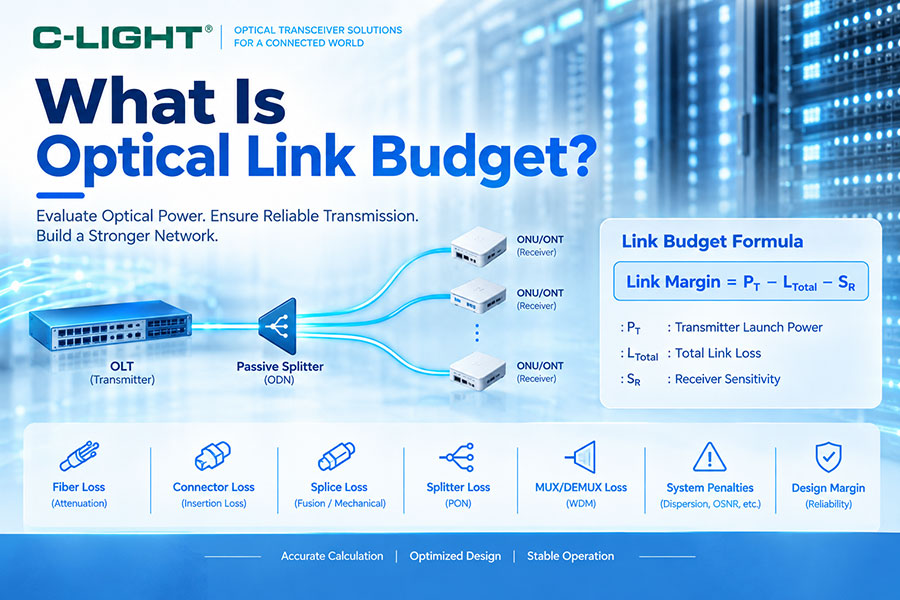
In any fiber optic communication system, the transmitter must deliver enough optical power to the receiver after the signal passes through fiber, connectors, splices, splitters, multiplexers, and other passive components. The optical link budget is the engineering method used to quantify this relationship. By comparing the available transmitter output power with the total optical loss and the receiver's minimum required input power, engineers can determine whether a link has sufficient margin for reliable operation. Link budget analysis is therefore a fundamental step in designing Ethernet, telecom, PON, WDM, data center interconnect, and long-distance optical networks.
1. What Is Optical Link Budget?
Optical link budget is the amount of optical power available to overcome all transmission losses between an optical transmitter and receiver while still keeping the received signal within the required operating range.
The basic relationship can be expressed as:
Optical Link Margin = Transmitter Launch Power − Total Link Loss − Receiver Sensitivity Requirement
A positive link margin indicates that the receiver should have sufficient optical power under the assumed conditions. In practical engineering, an additional design margin is normally reserved for aging, temperature variation, connector contamination, repair activity, and other uncertainties.
2. Why Is Optical Link Budget Important?
Optical power alone does not determine whether a communication link will work. A transmitter with high output power may still fail to provide a reliable link if fiber attenuation, connector loss, splitter loss, or other penalties consume most of the available power.
Link budget analysis allows engineers to determine the maximum supported distance, select an appropriate optical transceiver, evaluate passive network components, and verify whether sufficient margin remains after deployment.
3. The Main Parameters of an Optical Link Budget
A typical optical link budget is based on several key parameters: transmitter output power, receiver sensitivity, fiber attenuation, connector loss, splice loss, passive component loss, optical penalties, and design margin.
These parameters are usually evaluated at the wavelengths and operating conditions relevant to the selected transceiver and fiber system.
4. What Is Transmitter Launch Power?
Transmitter launch power is the optical power coupled from the transmitter into the fiber. It is usually specified in dBm and may be given as a typical value, minimum value, or maximum value.
For conservative link-budget calculations, the minimum guaranteed transmitter launch power is generally more useful than a typical value because it represents a lower-power operating condition.
5. What Is Receiver Sensitivity?
Receiver sensitivity is the minimum optical power required at the receiver input to achieve the specified performance, typically at a defined bit error rate or other performance threshold.
For example, if a receiver sensitivity is specified as -18 dBm, the received optical power must generally remain above this threshold for the receiver to meet its specified performance under the defined test conditions.
6. What Is Optical Power Budget?
Optical power budget is commonly calculated from the transmitter power and receiver sensitivity:
Available Optical Budget = Minimum Transmitter Launch Power − Receiver Sensitivity
Because dBm values are logarithmic, subtraction between launch power and sensitivity produces a budget in dB. This available budget is then consumed by fiber loss, connectors, splices, passive components, system penalties, and engineering margin.
7. What Is Fiber Attenuation?
Fiber attenuation represents the reduction in optical power as light propagates through the fiber. It is normally expressed in dB/km and depends on the fiber type, wavelength, temperature, bending condition, and installation quality.
The basic fiber-loss calculation is:
Fiber Loss = Fiber Attenuation × Fiber Length
For example, if the attenuation is 0.35 dB/km and the fiber length is 20 km, the nominal fiber loss is 7 dB before other losses are added.
8. What Is Connector Loss?
Every mated fiber connector introduces insertion loss. A link may contain connectors at the transceiver, patch panel, splice enclosure, optical distribution frame, or other connection points.
Connector loss should be calculated according to the actual number of connector pairs and the specified or measured insertion loss. Using an unrealistically low connector-loss assumption can produce an overoptimistic link budget.
9. What Is Splice Loss?
Fusion splicing and mechanical splicing introduce additional optical loss. Fusion splice loss is typically much lower than connector loss, but the cumulative effect of many splices can become important in long-distance or high-loss links.
A complete budget should therefore account for the expected number of splices and the corresponding loss per splice.
10. What Is Optical Splitter Loss?
Optical splitters are especially important in PON networks because they intentionally divide optical power among multiple branches. The split ratio has a direct effect on insertion loss.
As the split ratio increases, the available power per output branch decreases. For this reason, PON systems require careful coordination between splitter loss, fiber loss, connector loss, transceiver output power, receiver sensitivity, and the selected optical budget class.
11. What Is MUX/DEMUX Loss?
WDM systems introduce additional optical losses through multiplexers and demultiplexers. The insertion loss of a MUX/DEMUX depends on the optical architecture, number of channels, wavelength plan, component technology, and operating wavelength.
In DWDM systems, MUX/DEMUX loss must be considered together with amplifier gain, channel power balance, wavelength-dependent loss, and other system-level parameters.
12. What Is Optical Link Margin?
Optical link margin is the remaining optical budget after all expected link losses and required penalties have been accounted for.
A practical expression is:
Link Margin = Available Optical Budget − Total System Losses − Design Margin
A link with a very small remaining margin may operate under ideal laboratory conditions but become unstable when temperature, connector contamination, fiber repair, component aging, or additional deployment loss is introduced.
13. What Is Design Margin?
Design margin is an additional allowance reserved for uncertainties that may not be fully represented in the nominal link-loss calculation. It is not a substitute for accurate engineering; instead, it protects the link against foreseeable variations during operation.
Factors that may justify additional margin include connector degradation, temperature effects, fiber aging, future patching, installation variation, and uncertainty in component specifications.
14. What Is the Difference Between Link Budget and Link Margin?
Link budget refers to the total amount of optical loss that the system can theoretically tolerate based on transmitter and receiver specifications. Link margin is the amount of budget that remains after the actual or estimated link losses are deducted.
For example, a transceiver may provide a 10 dB available optical budget, while the deployed path may consume 7 dB. The resulting nominal link margin is 3 dB before any additional engineering allowance is considered.
15. Optical Link Budget Calculation Example
Consider a single-mode fiber link with the following simplified parameters:
| Parameter | Value |
|---|---|
| Minimum Transmitter Launch Power | -2 dBm |
| Receiver Sensitivity | -18 dBm |
| Fiber Length | 20 km |
| Fiber Attenuation | 0.35 dB/km |
| Connector Loss | 1.0 dB total |
| Splice Loss | 0.5 dB total |
The available optical budget is:
-2 dBm − (-18 dBm) = 16 dB
Fiber loss is:
20 km × 0.35 dB/km = 7 dB
The estimated total passive loss is:
7 dB + 1.0 dB + 0.5 dB = 8.5 dB
The remaining nominal budget is therefore:
16 dB − 8.5 dB = 7.5 dB
This simplified example shows why link-budget analysis must consider the complete optical path rather than transmission distance alone.
16. What Are Optical Penalties?
Not every performance limitation appears as physical insertion loss. High-speed optical systems can also experience penalties caused by chromatic dispersion, modal effects, reflections, extinction-ratio limitations, transmitter distortion, receiver effects, polarization-related effects, and other impairments.
In a detailed system design, these penalties may be included as additional dB terms or evaluated through system-level performance measurements such as BER, eye diagrams, or receiver sensitivity testing.
17. Link Budget and High-Speed Optical Transceivers
At 100G, 400G, 800G, and higher data rates, link budget analysis becomes more closely connected with transceiver architecture and modulation technology. PAM4 systems, for example, have tighter signal-quality requirements than conventional NRZ systems and must be evaluated using more than simple optical power measurements.
Receiver sensitivity, transmitter optical performance, dispersion, equalization, FEC, and electrical channel characteristics can all influence the usable system margin.
18. Link Budget for 100G, 400G, and 800G Links
The nominal optical budget of a transceiver depends on its exact specification rather than simply its data rate. A 400G or 800G module designed for a few hundred meters may have a completely different optical budget from a long-reach 400G or 800G module designed for several kilometers.
Therefore, transceiver selection should always be based on the specified transmitter output power, receiver sensitivity, supported fiber type, maximum reach, connector configuration, and operating conditions.
19. Optical Link Budget in PON Networks
PON link-budget engineering is more complex than a simple point-to-point fiber connection because one OLT port can serve multiple ONU or ONT endpoints through passive splitting.
The calculation must account for feeder fiber, distribution fiber, splitter insertion loss, connector loss, splice loss, optical distribution components, and the specific power budget supported by the PON technology.
20. Optical Link Budget in CWDM and DWDM Networks
WDM systems require additional analysis because optical channels share the same fiber infrastructure. Besides fiber and connector losses, engineers must consider MUX/DEMUX insertion loss, wavelength-dependent loss, channel isolation, amplifier gain where applicable, and power balance across wavelengths.
DWDM networks can also require analysis of optical signal-to-noise ratio, nonlinear effects, dispersion, and amplifier performance, especially for long-haul systems.
21. Optical Link Budget vs. Fiber Distance
Maximum transmission distance cannot be determined from fiber attenuation alone. It depends on the available optical budget and the total loss per unit length, together with fixed losses and system penalties.
A useful conceptual relationship is:
Maximum Reach ≈ (Available Budget − Fixed Losses − Required Margin) ÷ Fiber Attenuation
In real networks, the result should be validated against the transceiver's specified maximum reach and the relevant optical standards.
22. What Happens When the Link Budget Is Too Low?
If total optical loss exceeds the available budget, the receiver may not receive sufficient optical power. The result can be unstable operation, increased bit errors, link flapping, packet loss, or complete loss of connectivity.
Adding a higher-power optical module is not always the correct solution. Excessive received power can also overload a receiver, so both minimum and maximum receiver input power limits must be checked.
23. What Happens When Received Optical Power Is Too High?
Optical systems are not designed simply to maximize received power. A receiver has an overload limit, and excessive optical input can degrade receiver performance or prevent correct operation.
For this reason, a proper optical design must satisfy both conditions: the received power must remain above the required sensitivity and below the receiver overload limit.
24. Link Budget and DOM/DDM Monitoring
Digital Optical Monitoring (DOM) or Digital Diagnostic Monitoring (DDM) can provide real-time information such as transmitter optical power, receiver optical power, module temperature, supply voltage, and laser bias current.
These measurements can help engineers compare actual operating conditions with the original link-budget assumptions and identify abnormal loss or degradation in deployed networks.
25. How to Perform an Optical Link Budget Analysis?
A practical analysis normally starts by identifying the exact transmitter and receiver specifications. The next step is to map the complete optical path and list every loss source, including fiber, connectors, splices, splitters, MUX/DEMUX devices, and other passive components.
After calculating total loss, the result is compared with the available optical budget. A suitable engineering margin is then included, and the final design is validated against the transceiver's specified operating range and actual field conditions.
26. Optical Link Budget Best Practices
Use guaranteed minimum transmitter power and the specified receiver sensitivity rather than relying only on typical values. Measure or use realistic insertion-loss values for passive components, count every connector and splice, include the actual fiber length, and reserve an appropriate design margin.
For high-speed and long-distance systems, power-budget analysis should also be combined with BER, dispersion, OSNR, eye-diagram, and other relevant system-level validation methods.
27. Optical Link Budget FAQ
Q1. What is an optical link budget?
Q2. How is optical link budget calculated?
Q3. What is the difference between optical budget and link margin?
Q4. Does a longer fiber always require a higher-power optical module?
Q5. Can too much optical power cause problems?
Q6. Is optical link budget important for 400G and 800G?
28. Summary
Optical link budget is a fundamental method for evaluating whether an optical communication link can operate reliably across its intended transmission path. The calculation must consider transmitter launch power, receiver sensitivity, fiber attenuation, connectors, splices, splitters, MUX/DEMUX components, system penalties, and engineering margin. As networks move toward 100G, 400G, 800G, and beyond, accurate optical-budget analysis becomes increasingly important for transceiver selection, network design, troubleshooting, and long-term link reliability.
 >
>

 >
>
 >
>
 >
>
 >
>
 >
>
 >
>
 >
>