TEL:+86 132 6656 7067




Optical transceivers are available in different transmission distances to support a wide range of data center, enterprise, campus and telecom applications. Among single-mode optical solutions, 2km and 10km modules are commonly selected for links that require more reach than short-range optics.
The most obvious difference between a 2km and 10km optical transceiver is transmission distance. However, the difference extends to optical power budget, fiber loss, transmitter and receiver design, component selection, power consumption, cost and deployment scenarios. Understanding these factors helps network designers select a module that matches the actual link requirements.
1. 2km vs 10km Optical Transceiver at a Glance
| Feature | 2km Optical Transceiver | 10km Optical Transceiver |
|---|---|---|
| Typical Maximum Reach | Up to about 2km | Up to about 10km |
| Typical Fiber | Commonly single-mode fiber | Commonly single-mode fiber |
| Optical Budget | Lower | Higher |
| Transmission Environment | Short-to-medium single-mode links | Longer single-mode links |
| Optical Components | Optimized for moderate reach | Designed for greater optical reach |
| Power Consumption | Often lower | Often higher |
| Cost | Generally lower | Generally higher |
| Typical Applications | Data centers, campuses and inter-building links | Long campus, metro and other extended links |
2. What Is a 2km Optical Transceiver?
A 2km optical transceiver is designed to support optical communication over links with a target reach of approximately 2 kilometers under specified operating conditions.
At many modern Ethernet speeds, 2km solutions are associated with single-mode fiber and are positioned between very short-reach data center optics and longer-reach telecom-style modules. The exact specification depends on the data rate, wavelength, optical architecture and standard supported by the module.
3. What Is a 10km Optical Transceiver?
A 10km optical transceiver is designed for optical links extending up to approximately 10 kilometers. Because the transmission path is significantly longer, the module needs enough optical budget to compensate for fiber attenuation and connection losses.
10km optics are commonly used when the network extends beyond typical data center distances and requires longer single-mode fiber connectivity.
4. The Main Difference Is Transmission Distance
The primary distinction is the supported reach. A 2km optical transceiver is designed around a much shorter link budget, while a 10km optical transceiver must maintain reliable operation over a substantially longer optical path.
The reach rating is not simply a theoretical number. It reflects the relationship between transmitter output power, receiver sensitivity, fiber attenuation, connector loss and the required operating margin.
5. Optical Power Budget
Optical power budget is one of the most important differences between 2km and 10km modules.
A simplified link-budget calculation is:
Maximum Allowable Loss = Transmitter Output Power − Receiver Sensitivity
A 10km module generally provides a larger optical budget than a 2km module because the longer link introduces more fiber attenuation and potentially more connection losses.
For an actual deployment, the module datasheet should be used to determine the specified transmit power, receiver sensitivity and supported link margin.
6. Fiber Loss and Link Distance
Fiber attenuation increases as the optical path becomes longer. A 2km link therefore has significantly less fiber loss than a 10km link using the same fiber characteristics.
A simplified total-loss model can be written as:
Total System Loss = Fiber Loss + Connector Loss + Passive Device Loss + Other Link Losses
This difference explains why a 10km optical transceiver requires a higher-performance optical design than an equivalent 2km solution.
7. Fiber Type
Both 2km and 10km high-speed optical modules are commonly designed for single-mode fiber. Single-mode fiber provides the transmission characteristics needed for longer optical links and is widely used for extended Ethernet connections.
However, the fiber type should always be verified against the specific transceiver specification. The module's wavelength, connector configuration and supported fiber type must all be compatible with the installed fiber infrastructure.
8. Wavelength and Optical Architecture
Wavelength selection depends on the network standard and transceiver architecture. Many 2km and 10km single-mode Ethernet solutions operate around the 1310nm window, while some longer-reach technologies use other wavelength ranges depending on the application.
The optical architecture may also differ. A 2km module can be designed with a simpler optical budget, while a 10km module may require higher-performance transmitters, receivers or other optical components to maintain the required link margin.
9. Laser Technology
The transmitter technology is determined by the specific data rate and optical architecture rather than by distance alone. Directly modulated lasers and externally modulated laser technologies can both appear in high-speed optical transceiver designs.
For longer-reach applications, the module designer must consider transmitter output, extinction characteristics, receiver sensitivity, dispersion effects and overall signal integrity.
10. 2km vs 10km Optical Transceiver Cost
A 2km optical transceiver is generally less expensive than a comparable 10km module. The difference is related to optical budget, component requirements and the complexity needed to support the longer transmission distance.
For large deployments, selecting a 10km module when the network only requires 2km may increase equipment cost without providing a corresponding operational benefit.
11. Power Consumption
Power consumption varies significantly according to data rate, form factor, DSP architecture and optical components. In comparable module families, longer-reach optics may require more optical power or more complex components, which can increase power consumption.
This consideration becomes particularly important in high-density data centers where thousands of transceivers may be installed in switches and servers.
12. 2km Optical Transceiver Applications
2km optical transceivers are commonly used for connections that exceed the reach of short-range modules but do not require a 10km optical budget.
Typical applications include data center interconnects, row-to-row links, campus networks, equipment-room connections and building-to-building links where the optical path remains within the supported 2km range.
13. 10km Optical Transceiver Applications
10km optical transceivers are intended for longer optical connections. They can be used where network devices are separated by several kilometers or where a larger optical margin is needed for the planned fiber route.
Typical applications include extended campus networks, inter-building connections, data center interconnects and selected metro or service-provider network scenarios.
14. 2km vs 10km in Data Centers
Modern data centers often use a combination of short-, medium- and long-reach optical modules. A 2km module can cover many internal connections, especially when racks, rows or buildings are relatively close together.
A 10km module is useful when the optical path extends across a larger facility or between separate sites. The choice should be based on the complete fiber route rather than simply the straight-line distance between two devices.
15. 400G Example: FR4 vs LR4
400G Ethernet provides a useful example of the difference between approximately 2km and 10km optical solutions.
400GBASE-FR4 is specified for single-mode fiber links of at least 2km using four WDM lanes. 400GBASE-LR4 is associated with longer 10km-class single-mode links and a higher optical budget.
| 400G Interface | Typical Reach | Fiber | Positioning |
|---|---|---|---|
| 400GBASE-FR4 | Up to at least 2km | SMF | Shorter single-mode reach |
| 400GBASE-LR4 | Up to about 10km | SMF | Longer single-mode reach |
16. 100G Example: FR1 vs LR1
The same reach distinction can be seen in 100G Ethernet. 100GBASE-FR1 is designed for single-mode transmission over at least 2km, while 100GBASE-LR1 supports single-mode transmission over at least 10km.
These interfaces demonstrate that increasing reach can require a different optical budget even when the nominal Ethernet data rate remains the same.
17. Why a 10km Module Is Not Simply a Longer 2km Module
A 10km module cannot be considered simply a 2km module with a higher distance label. The module must maintain sufficient optical performance throughout the longer link.
This can affect transmitter power, receiver sensitivity, wavelength control, optical components, monitoring and overall module design. The exact differences depend on the specific transceiver family.
18. Can a 10km Transceiver Be Used on a 2km Link?
In many cases, a 10km-rated transceiver can operate over a shorter 2km link when the optical interface and system specifications are compatible.
However, using a 10km module on a 2km link may not be economically efficient. The additional optical capability may not provide a practical advantage when a lower-cost 2km solution already meets the link requirements.
19. Can a 2km Transceiver Be Used on a 10km Link?
A 2km-rated transceiver should not be assumed to support a 10km connection. The optical budget may be insufficient to overcome the additional fiber and connection losses.
Operating beyond the manufacturer's specified reach can reduce link margin and may result in unreliable communication. The module datasheet and calculated link budget should therefore be checked before deployment.
20. Optical Margin Is Critical
Network planning should not stop at the nominal transmission distance. A real fiber route may contain patch panels, connectors, adapters, splices and passive components that add optical loss.
A useful design should maintain sufficient margin after accounting for the complete optical path. This becomes especially important for 10km links because a larger portion of the optical budget is already consumed by fiber attenuation.
21. 2km vs 10km: Deployment Considerations
| Requirement | 2km Solution | 10km Solution |
|---|---|---|
| Link under 2km | Usually sufficient when the budget is adequate | May provide unnecessary additional reach |
| Link between 2km and 10km | Usually insufficient | More suitable |
| Longer campus connection | Depends on actual route | Often appropriate |
| Optical budget requirement | Moderate | Higher |
| Cost sensitivity | Generally more economical | Generally higher cost |
| Future longer-distance deployment | Limited by rated reach | Provides greater reach capability |
22. How to Choose Between 2km and 10km Optical Transceivers
The first step is to calculate the complete optical path. Consider the physical distance, fiber attenuation, number of connectors, patch points, passive devices and required safety margin.
Next, verify the data rate and interface standard. A 2km and 10km module may use different standards even when the host port has the same form factor.
Finally, compare optical budget, power consumption, cost and equipment compatibility. The selected module should meet the required reach while maintaining adequate operating margin.
23. 2km vs 10km Optical Transceiver: Summary
2km and 10km optical transceivers are designed for different transmission-distance requirements. A 2km module is generally suited to shorter single-mode links, while a 10km module is designed for substantially longer connections and therefore requires a larger optical budget.
The difference affects fiber infrastructure, optical components, power consumption and cost. 2km solutions are often appropriate for shorter data center and campus connections, while 10km optics provide greater flexibility for extended links.
The correct choice should be based on actual link distance, optical loss, fiber type, interface standard, optical margin and equipment compatibility rather than reach alone.
 >
>

 >
>
 >
>
 >
>
 >
>
 >
>
 >
>
 >
>