TEL:+86 132 6656 7067





In fiber optic networks, a stable connection depends on whether enough optical power reaches the receiving transceiver after traveling through the entire fiber path. Fiber attenuation, connectors, fusion splices, patch panels, and passive optical devices all contribute to signal loss. An optical link budget brings these factors together to determine whether a proposed connection has sufficient power margin for reliable operation.
Core calculation: Subtract the receiver's minimum sensitivity from the transmitter's minimum output power to obtain the available optical power budget. Then subtract all expected link losses and the required operating margin. A positive remaining margin indicates that the link meets the planned power-loss requirement, provided other optical performance limits are also satisfied.
1. What Is an Optical Link Budget?
An optical link budget is the calculation of the maximum allowable optical loss between a transmitter and a receiver. It establishes whether the received signal can remain above the receiver sensitivity threshold after accounting for the losses introduced by the fiber infrastructure.
The calculation starts with two transceiver specifications:
Minimum transmitter output power: The lowest optical power the transmitter is specified to deliver under its defined operating conditions.
Receiver sensitivity: The minimum received optical power at which the receiver meets its specified performance, usually under a defined bit error rate and test condition.
For example, if a transceiver has a minimum transmitter output power of -3 dBm and a receiver sensitivity of -18 dBm:
The available optical power budget is therefore 15 dB. This means the total allowable optical loss cannot exceed 15 dB before considering any additional design reserve or specified penalties.
2. Identify Every Source of Optical Link Loss
The total link loss is the sum of the attenuation and insertion losses encountered along the optical path. A complete calculation should account for the actual installed topology rather than using fiber length alone.
| Loss Source | Calculation Method | What to Include |
|---|---|---|
| Fiber attenuation | Fiber length × attenuation per kilometer | Actual cable length and the attenuation specification at the operating wavelength |
| Connector insertion loss | Number of mated connection pairs × loss per pair | Equipment interfaces, patch panels, adapters, and intermediate connections |
| Fusion splice loss | Number of splices × loss per splice | All fusion splices along the route |
| Passive component loss | Sum of specified insertion losses | Splitters, WDM filters, muxes, demuxes, and other passive devices |
| Additional optical penalties | Use applicable system specifications | Dispersion, reflections, or other specified penalties where relevant |
| Engineering margin | Reserved design allowance | Future repairs, aging, environmental variation, and measurement uncertainty |
Fiber attenuation is usually expressed in dB/km. It varies with fiber type and wavelength. For example, single-mode fiber typically has lower attenuation around 1550 nm than at 1310 nm, although the actual value must be taken from the cable specification or measured link.
Connector and splice losses should also be based on actual component specifications or test results. A connector pair is one mated connection between two connectorized ends; do not count each connector ferrule as a separate mated pair.
3. The Complete Optical Link Budget Formula
A practical calculation separates the available power budget, the physical link loss, and the reserved engineering margin.
Fiber loss is calculated as:
The remaining power margin is:
If a separate engineering reserve is required, subtract it as well:
A positive design margin means the link has remaining power headroom after the planned reserve. A zero or negative result means the design does not meet the selected margin requirement.
4. Worked Example: Calculate a 20 km Single-Mode Fiber Link
Consider a hypothetical 10G optical link using single-mode fiber. The following values are illustrative and are not specifications for a particular C-LIGHT product.
| Parameter | Assumed Value |
|---|---|
| Minimum transmitter output power | -3 dBm |
| Receiver sensitivity | -18 dBm |
| Fiber length | 20 km |
| Fiber attenuation | 0.25 dB/km |
| Mated connector pairs | 4 |
| Loss per connector pair | 0.50 dB |
| Fusion splices | 6 |
| Loss per fusion splice | 0.10 dB |
| Other passive component loss | 1.50 dB |
| Reserved engineering margin | 3.00 dB |
Step 1: Calculate the available optical power budget.
Step 2: Calculate fiber attenuation.
Step 3: Calculate connector loss.
Step 4: Calculate splice loss.
Step 5: Add all physical link losses.
Step 6: Calculate the remaining margin.
Step 7: Subtract the reserved engineering margin.
Result: The illustrative link has 2.90 dB of remaining design margin after reserving 3 dB. Its calculated physical loss is 9.10 dB, compared with an available power budget of 15 dB. The design meets the assumed power-margin target, subject to receiver overload and other optical performance checks.
5. Calculate the Expected Received Optical Power
Another useful way to evaluate the link is to estimate the received optical power using the transmitter's minimum output power and the total physical link loss.
Using the previous example:
The expected received power is -12.10 dBm. The receiver sensitivity is -18 dBm, so the difference is:
This is the actual calculated power margin before reserving the additional 3 dB engineering allowance. It is useful to compare this result with live DOM/DDM readings after installation.
6. Check Receiver Overload as Well as Sensitivity
A link can have enough optical power to exceed receiver sensitivity and still operate outside the receiver's acceptable input range. If the received signal is too strong, the receiver may become overloaded or experience performance degradation.
For this reason, the design should check both ends of the receiver's operating range:
Minimum received power: Must remain at or above the receiver sensitivity requirement after accounting for worst-case loss.
Maximum received power: Must not exceed the receiver's specified overload limit under the lowest-loss operating condition.
| Receiver Check | Design Requirement | Potential Issue |
|---|---|---|
| Receiver sensitivity | Received power must be sufficiently high | Weak signal, errors, or link instability |
| Receiver overload | Received power must remain below the maximum input limit | Receiver overload or degraded performance |
| Operating range | Received power must stay within the specified range | Unreliable operation across changing conditions |
This check is particularly important when using high-output long-reach transceivers over short fiber links. An optical attenuator may be required in some applications, but its value should be selected according to the transmitter output, receiver overload limit, and complete link specifications.
7. Special Considerations for PON and DWDM Links
Not all optical networks can be evaluated using only the simple point-to-point fiber formula. Passive optical networks and wavelength-division multiplexing systems introduce additional components and performance constraints.
PON networks:
GPON and XGS-PON optical distribution networks include passive splitters that introduce significant insertion loss. The splitter loss depends on the split ratio and the component's actual specifications. Both downstream and upstream directions must be evaluated independently because they use different transmitters, receivers, and operating wavelengths.
For a PON design, include the feeder fiber, distribution fiber, drop fiber, splitter insertion loss, connector loss, splice loss, and the applicable optical class limits. A higher split ratio generally increases splitter loss and reduces the power available to each optical network terminal.
DWDM networks:
DWDM systems include muxes, demuxes, optical amplifiers, filters, and sometimes ROADMs. Their design must account for passive insertion loss, amplifier gain, amplifier noise, channel power, and optical signal-to-noise ratio (OSNR). A basic power budget remains useful, but it cannot by itself prove that a coherent or amplified DWDM link will meet its performance target.
8. How to Measure and Verify an Optical Link Budget
A theoretical calculation should be checked against the installed fiber plant. Actual connector condition, splice quality, cable routing, and passive component losses can differ from initial assumptions.
Review transceiver specifications: Record minimum and maximum transmitter power, receiver sensitivity, overload limit, wavelength, and any specified optical penalties.
Confirm the fiber route: Identify the fiber type, total length, connection points, splice locations, and passive components.
Inspect connector end faces: Contamination and damage can increase insertion loss or cause unstable optical performance.
Measure end-to-end insertion loss: Use a calibrated optical loss test set or light source and power meter at the appropriate wavelength.
Use OTDR for route diagnostics: An OTDR can identify fiber events, estimate event loss, and locate breaks or abnormal attenuation.
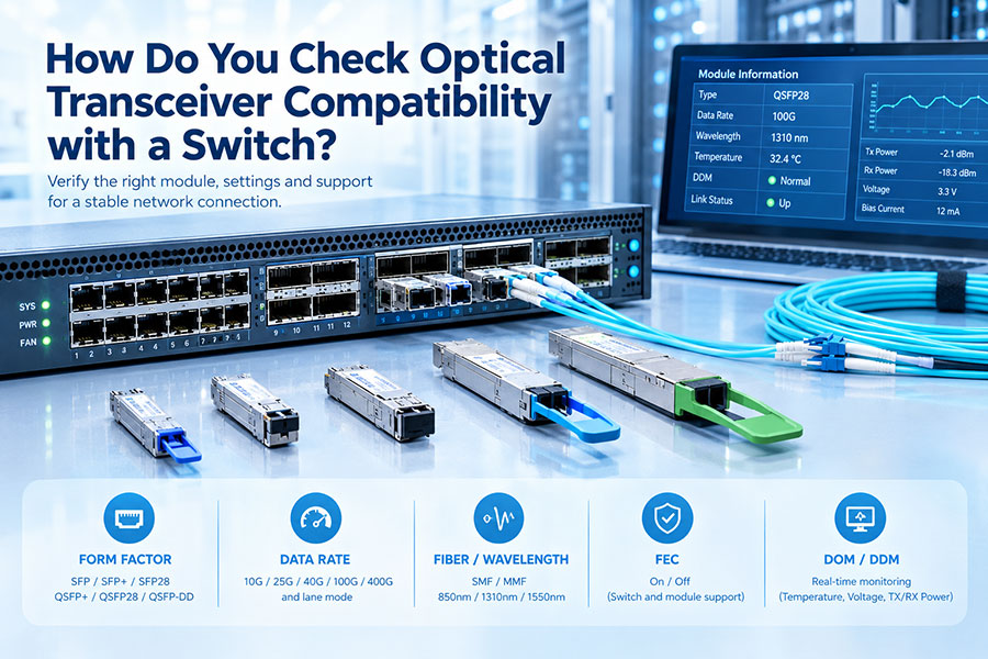
Check live optical power: Review DOM/DDM measurements where supported by the transceiver and host equipment.
Verify actual link performance: Check alarms, error counters, FEC statistics where applicable, and stability under normal operating conditions.
An optical power meter measures received optical power, while an OTDR provides information about the fiber route and individual events. These tools serve different purposes. An OTDR trace alone should not be treated as a replacement for end-to-end insertion-loss testing.
9. Common Optical Link Budget Calculation Mistakes
| Common Mistake | Why It Causes Problems | Better Approach |
|---|---|---|
| Using typical TX power instead of minimum TX power | Can overestimate the available budget | Use the guaranteed minimum transmitter specification |
| Ignoring connector pairs | Underestimates total insertion loss | Count each actual mated connection |
| Ignoring splitter or WDM loss | Can substantially overestimate available receive power | Include each passive component's specified insertion loss |
| Using attenuation at the wrong wavelength | Produces an inaccurate fiber-loss estimate | Use attenuation data for the operating wavelength |
| Confusing dB and dBm | Leads to incorrect calculations | Keep absolute power and relative loss units distinct |
| Ignoring receiver overload | A strong signal may exceed the receiver's input range | Check both sensitivity and maximum input power |
| Using power budget as the only qualification | Does not account for all signal-quality limitations | Check dispersion, OSNR, FEC, and interface requirements where applicable |
10. Optical Transceiver Selection for Different Link Budgets
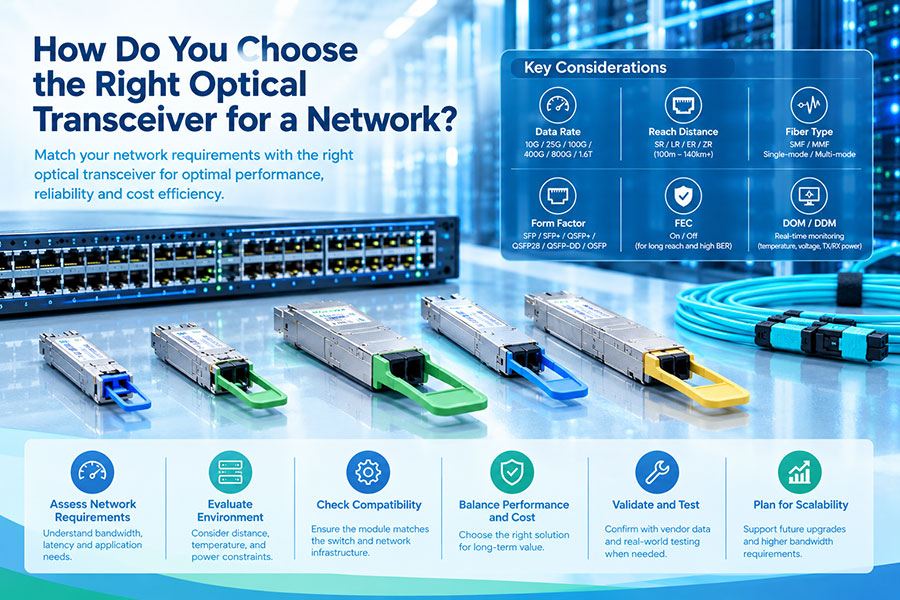
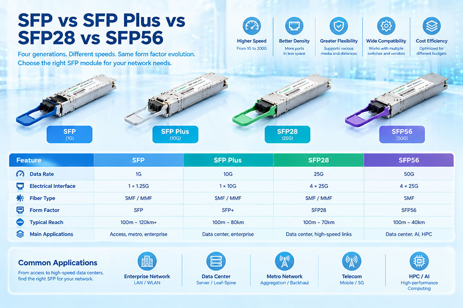
The calculated link budget helps determine which optical interface is appropriate for a particular network route. The selected transceiver must support the required data rate, fiber type, wavelength, connector arrangement, and transmission distance.
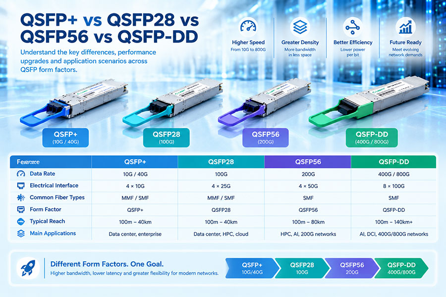
For high-speed network infrastructure, C-LIGHT offers optical transceiver product families covering 400G and 800G platforms. These products include different optical application types, so the exact model specification should be checked before matching a transceiver to a calculated link budget.
400G QSFP-DD Optical Transceivers
A high-density platform for 400G switching and data center connectivity. Select the specific SR, DR, FR, or other supported optical interface according to the fiber route and link-loss calculation.
View 400G QSFP-DD Products400G OSFP Optical Transceivers
Designed for high-capacity switching and data center infrastructure. The optical power range, receiver sensitivity, and supported reach depend on the selected module variant.
View 400G OSFP Products800G QSFP-DD Optical Transceivers
An 800G platform for next-generation data center networks. Verify the selected optical application, lane configuration, fiber type, and link budget before deployment.
View 800G QSFP-DD Products800G OSFP Optical Transceivers
High-speed optical connectivity for advanced switching and AI data center infrastructure. Different reach options require different optical link specifications.
View 800G OSFP ProductsA transceiver's form factor or data rate does not establish its link budget. Always use the exact product datasheet to obtain minimum TX power, receiver sensitivity, overload limits, and other applicable parameters. For links using different models at each end, verify the optical specifications in both directions.
11. Conclusion: Calculate Loss, Margin, and Receiver Limits
Optical link budget calculation is an essential part of fiber network planning. Start with the minimum transmitter output power and receiver sensitivity to determine the available optical power budget. Calculate fiber attenuation, connector loss, splice loss, and passive component insertion loss, then subtract the applicable penalties and reserved engineering margin.
A reliable design must also confirm that received power does not exceed the receiver's overload limit. For higher-capacity or more complex systems, additional checks for dispersion, OSNR, FEC, and interface-specific requirements are necessary.
By combining datasheet specifications with accurate fiber measurements, network engineers can select suitable optical transceivers, identify insufficient power margin before deployment, and reduce the risk of unstable optical links.
Available optical power budget equals minimum transmitter output power minus receiver sensitivity. The remaining margin is calculated by subtracting total link loss and applicable penalties from that budget.
A 3 dB reserve is commonly used as a planning allowance in many controlled fiber links, but the appropriate value depends on the network design, installation environment, equipment specifications, and applicable standards. Some systems require different margins.
dBm expresses absolute optical power relative to 1 mW. dB expresses a relative gain or loss. Transmitter power and receiver sensitivity are generally expressed in dBm, while fiber attenuation and insertion loss are expressed in dB.
No. A higher budget can allow greater total optical loss, but dispersion, OSNR, receiver overload, nonlinear effects, and the transceiver's specified reach can still limit the connection.
No. DOM/DDM provides live monitoring information such as received optical power, transmitter power, temperature, and voltage when supported. It is useful for checking an installed link, but it does not replace design calculations or end-to-end loss testing.
Planning a high-speed optical network?
Choose optical transceivers according to the required data rate, transmission distance, fiber infrastructure, and link budget.
Contact C-LIGHT >

 >
 >
 >
 >
 >
 >
 >