TEL:+86 132 6656 7067





An industrial fiber link can pass traffic successfully during initial installation and still develop problems after months of operation. Connector contamination, additional patch panels, temperature-related optical changes, cable repairs and aging components can gradually consume the available optical margin. These issues are particularly important in remote industrial networks, where links may operate continuously and physical maintenance can be difficult.
An optical link budget provides a quantitative way to evaluate whether a transceiver can deliver enough optical power to its receiver after all losses in the fiber route are considered. However, a reliable industrial link design must go beyond the basic difference between transmitter output power and receiver sensitivity. It must also account for receiver overload, engineering margin, operating temperature, signal quality and the actual condition of the installed fiber.
Evaluating these parameters before deployment helps engineers determine whether a proposed transceiver pair is suitable for the intended distance and operating environment, rather than relying solely on the transmission distance printed in a product description.
1. What Is an Industrial Optical Transceiver Link Budget?
An optical link budget is a system-level calculation that compares the optical power available from the transmitter with the power required by the receiver. It considers the loss introduced by fiber, connectors, splices and other components along the optical path.
The starting point is the optical power budget, which is the difference between transmitter output power and receiver sensitivity.
Power Budget (dB) = Minimum TX Power (dBm) − Receiver Sensitivity (dBm)
For example, if a hypothetical transceiver has a minimum transmit power of -2dBm and receiver sensitivity of -10dBm, the nominal optical power budget is:
This means the link has a nominal allowance of 8dB between the transmitter's minimum output and the receiver's sensitivity threshold. It does not mean that the full 8dB can be consumed by fiber attenuation. Connector losses, splices, passive components and the required engineering margin must also be included.
For industrial applications, the calculation should use the transceiver specifications applicable to its required operating conditions. A link that meets the budget at room temperature may have less margin if transmitter output or receiver sensitivity changes at temperature extremes.
2. Understand the Difference Between dBm and dB
Incorrect use of dBm and dB can produce mistakes in link-budget calculations. Although the units are related, they describe different quantities.
| Unit | Meaning | Common Application |
|---|---|---|
| dBm | Absolute optical power referenced to 1 milliwatt. | Transmit power, received power and receiver sensitivity. |
| dB | Relative gain, attenuation or difference between power levels. | Fiber loss, connector insertion loss and optical power budget. |
| dB/km | Optical attenuation per kilometer. | Fiber attenuation calculations. |
When subtracting two optical power levels expressed in dBm, the result is a relative difference expressed in dB.
For example, subtracting a receiver sensitivity of -10dBm from a transmitter output of -2dBm produces an 8dB power budget. The result is not 8dBm because it represents a difference rather than an absolute power level.
3. Identify the Main Parameters in the Link Budget
A useful link-budget assessment requires several transmitter, receiver and fiber specifications. Each parameter contributes to a different part of the calculation.
| Parameter | Definition | Role in Link Evaluation |
|---|---|---|
| Minimum TX power | Lowest specified transmitter optical output under the defined conditions. | Used for the conservative received-power calculation. |
| Maximum TX power | Highest specified transmitter optical output. | Used when evaluating receiver overload risk. |
| Receiver sensitivity | Minimum optical input required for specified receiver performance. | Defines the lower boundary of the receiver's operating range. |
| Receiver overload | Maximum specified input power for compliant receiver operation. | Checks whether a low-loss link delivers excessive optical power. |
| Fiber attenuation | Optical loss per unit length, commonly expressed in dB/km. | Determines the loss accumulated along the fiber route. |
| Connector insertion loss | Optical loss at a mated connector interface. | Accounts for patch panels, adapters and equipment connections. |
| Splice loss | Loss introduced by fusion or mechanical splices. | Accounts for permanent joints along the route. |
| Passive component loss | Loss from splitters, filters, multiplexers and other optical components. | Accounts for additional elements in the optical path. |
| Engineering margin | Reserved allowance for uncertainty, aging, repairs and future changes. | Prevents the link from depending entirely on ideal calculated conditions. |
Use specifications from the exact transceiver model and applicable optical interface. Minimum transmit power, maximum transmit power, receiver sensitivity and receiver overload are separate limits and should not be substituted for one another.
4. Calculate Total Optical Path Loss
After establishing the available optical power budget, calculate the total loss between the transmitter and receiver. The calculation should reflect the actual physical route, including all intermediate connection points.
Total Loss = Fiber Loss + Connector Loss + Splice Loss + Other Applicable Losses
Fiber attenuation
Fiber attenuation is the optical power lost as the signal travels through the cable. It depends on the fiber specification, wavelength and installation condition.
Fiber Loss (dB) = Fiber Attenuation (dB/km) × Fiber Length (km)
For planning purposes, representative single-mode fiber attenuation values may be around 0.3–0.4dB/km near 1310nm and approximately 0.18–0.30dB/km around the 1550nm region, depending on the fiber specification and measurement conditions. These are illustrative ranges, not guaranteed values for every installed cable.
Use the cable manufacturer's attenuation specification or measured route loss wherever available. ITU-T G.652 defines important characteristics of conventional single-mode fiber, including attenuation and chromatic dispersion parameters.
Connector and splice losses
Each connector pair and splice can introduce additional optical loss. A route with multiple patch panels may consume a meaningful part of the available budget even when its fiber length is relatively short.
Include:
Both equipment-side connector interfaces.
Intermediate patch panels and cross-connects.
Fusion or mechanical splices.
Passive optical splitters and filters.
CWDM or DWDM mux and demux insertion loss.
Other optical components installed in the route.
Count the actual mated interfaces and splices. Avoid double-counting connections if the selected cable or end-to-end loss specification already includes them.
5. Calculate the Remaining Optical Margin
The remaining margin shows how much optical budget is available after the estimated path loss and the reserved engineering margin have been deducted.
Remaining Margin = Available Power Budget − Total Path Loss − Reserved Engineering Margin
A positive result means the calculated path retains some margin beyond the amount reserved for uncertainty and future changes. A negative result indicates that the design does not meet the chosen margin requirement and needs further investigation.
The engineering margin should reflect the specific network design, expected route changes, maintenance practices, component variation and applicable system requirements. There is no single margin value that is automatically correct for every industrial link.
6. Worked Example: Evaluating a 10km Single-Mode Link
Consider a hypothetical 10km single-mode fiber connection between two industrial switches. The following values are assumed for illustrating the link-budget calculation. They are not specifications for a particular transceiver model.
| Input Parameter | Assumed Value |
|---|---|
| Minimum transmitter output power | -2dBm |
| Receiver sensitivity | -10dBm |
| Fiber length | 10km |
| Fiber attenuation | 0.35dB/km |
| Total connector loss | 1.0dB |
| Total splice loss | 0.2dB |
| Reserved engineering margin | 2.0dB |
Step 1: Calculate the available optical power budget
The available nominal optical power budget is 8dB.
Step 2: Calculate fiber attenuation
The calculated fiber loss is 3.5dB.
Step 3: Calculate total path loss
The estimated total path loss is 4.7dB.
Step 4: Calculate the remaining margin
The calculated remaining margin is 1.3dB after reserving the assumed 2dB engineering margin. Under these assumptions, the link meets the selected power-budget requirement with 1.3dB of additional calculated margin.
This is a preliminary power-budget assessment rather than a complete standards-compliance determination. Dispersion, receiver performance, FEC requirements and other optical interface conditions must still be evaluated where applicable.
7. Check Receiver Overload on Short and Low-Loss Links
A link-budget calculation should not focus only on whether enough optical power reaches the receiver. Too much received power can also cause problems.
Receiver sensitivity defines the lower input-power boundary, while receiver overload defines the upper boundary. A valid link must operate between these limits under the relevant test conditions.
Maximum Received Power = Maximum TX Power − Minimum Path Loss
For a conservative overload check, use the applicable maximum transmitter output and the minimum expected path loss. Compare the result against the receiver's overload specification.
For a low-power check, use minimum transmitter output and maximum expected path loss. This verifies the receiver's sensitivity margin under the more demanding loss condition.
| Link Condition | Transmitter Value | Path-Loss Condition | Receiver Limit to Check |
|---|---|---|---|
| Minimum received power | Minimum TX power | Maximum expected loss | Receiver sensitivity |
| Maximum received power | Maximum TX power | Minimum expected loss | Receiver overload |
This distinction is particularly important when an extended-reach transceiver is used over a short connection. If the received signal exceeds the receiver's permitted input range, an appropriately specified optical attenuator may be required, subject to the module and system design.
8. Account for Temperature in Industrial Link-Budget Evaluation
Industrial optical modules may operate across wider temperature ranges than conventional commercial transceivers. Temperature can affect laser output, wavelength, receiver behavior and the electrical characteristics of internal components.
For an accurate industrial link budget, the relevant optical specifications should remain valid across the required operating temperature range.
| Temperature-Related Parameter | Potential Effect | What to Verify |
|---|---|---|
| Transmitter output power | Laser efficiency and operating characteristics can change. | Minimum and maximum TX power across the specified temperature range. |
| Receiver sensitivity | Photodetector and receiver electronics may respond differently. | Sensitivity specifications and test results at temperature limits. |
| Laser wavelength | Emission wavelength may shift with junction temperature. | Wavelength tolerance and channel requirements. |
| Module case temperature | Local heat and restricted airflow may raise module temperature. | Operating case-temperature range and host cooling conditions. |
| Diagnostic readings | Temperature and other internal measurements may change. | DDM/DOM monitoring accuracy and warning thresholds. |
For example, an optical link installed in an outdoor cabinet may have sufficient margin during room-temperature testing but less margin during high-temperature operation if transmitter output or receiver sensitivity changes.
Use guaranteed optical limits over the required operating conditions when the datasheet provides them. Typical room-temperature values should not be substituted for guaranteed minimum and maximum values in a worst-case calculation.
Also distinguish module case temperature from ambient temperature. The transceiver's internal self-heating and the host equipment's thermal design can cause the case temperature to differ from the surrounding air temperature.
9. Consider Dispersion and Signal Quality Beyond Optical Power
A positive optical power margin does not guarantee that a link will transmit data correctly. The signal can still be affected by chromatic dispersion, modal bandwidth, reflections, receiver characteristics and other impairments.
| Signal or Transmission Factor | Why It Matters | Relevant Evaluation |
|---|---|---|
| Chromatic dispersion | Different wavelength components travel at different speeds through the fiber. | Check the transceiver's dispersion tolerance and applicable interface limits. |
| Modal bandwidth | Different propagation modes in multimode fiber can limit the usable data rate and reach. | Verify fiber grade and the supported SR/SX interface reach. |
| Optical reflections | Reflected light can affect transmitter or receiver behavior in sensitive systems. | Review reflectance and return-loss requirements where applicable. |
| OSNR | Noise affects signal quality in amplified optical systems. | Evaluate optical signal-to-noise ratio for applicable WDM and amplified links. |
| BER | Measures the frequency of incorrectly received bits. | Test against the specified BER criterion. |
| FEC performance | Shows how effectively the system corrects transmission errors. | Review pre-FEC errors, corrected errors and uncorrectable errors where applicable. |
For higher-speed PAM4 interfaces, signal-quality measurements such as TDECQ, OMA and lane-level eye performance may be relevant. For lower-speed NRZ interfaces, the applicable transmitter and receiver requirements are different.
Engineering teams should follow the applicable interface specification rather than applying the same optical acceptance criteria to every module type.
10. Distinguish Optical Power Budget from the Complete Link Budget
The terms optical power budget and link budget are often used interchangeably, but they describe different levels of evaluation.
| Term | Scope | Purpose |
|---|---|---|
| Optical power budget | Difference between transmitter output power and receiver sensitivity. | Establishes the nominal optical loss that can be tolerated. |
| Link budget | System-level assessment of power, path loss, margin and performance constraints. | Determines whether the complete link can meet its operating requirements. |
| Engineering margin | Reserved allowance for uncertainty or degradation. | Provides protection against relying entirely on ideal calculated conditions. |
For procurement and network planning, calculate the nominal power budget first. Then document the route-loss assumptions, engineering reserve, temperature conditions and other performance requirements separately.
11. Common Link-Budget Calculation Mistakes
Small calculation errors can lead to a design that appears acceptable on paper but performs poorly after deployment.
| Common Mistake | Why It Is a Problem | Better Practice |
|---|---|---|
| Using typical TX power instead of minimum TX power | Can overestimate the available power budget. | Use the specified minimum for the conservative low-power calculation. |
| Ignoring connector and patch-panel losses | Underestimates total route loss. | Count the actual connection interfaces and include their loss. |
| Confusing dBm with dB | Produces incorrect calculations or reporting. | Use dBm for absolute power levels and dB for relative loss or differences. |
| Ignoring receiver overload | A low-loss link may deliver excessive optical power. | Perform a separate maximum-input-power check. |
| Assuming attenuation alone determines reach | Dispersion and signal quality may impose additional distance limits. | Check all applicable optical interface requirements. |
| Applying generic fiber attenuation values | Actual cable performance depends on fiber type and wavelength. | Use cable specifications or measured route loss. |
| Leaving out engineering margin | Normal variations or future repairs may consume the remaining budget. | Set a project-appropriate reserve based on documented design rules. |
| Mixing unrelated transmitter and receiver specifications | The values may refer to incompatible interfaces or test conditions. | Use specifications for the matched optical interface and operating conditions. |
| Counting the same loss twice | Can make the estimated path loss unnecessarily high. | Define the loss model and verify what each measurement already includes. |
12. Verify the Link Budget After Installation
A calculated link budget is a design estimate. Field measurement is necessary to determine whether the installed optical route behaves as expected.
A practical verification process includes:
Confirm the module models: Check the transceiver part numbers, optical interface and specified wavelength at both ends.
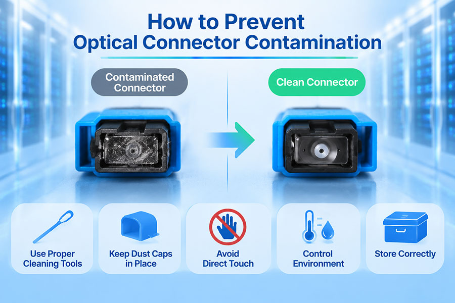
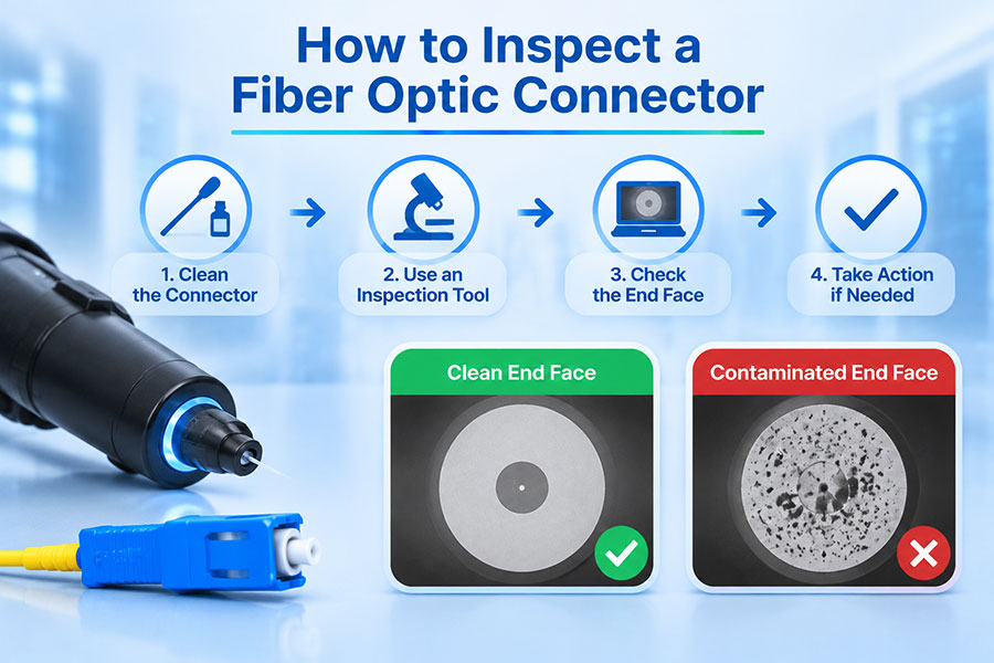
Inspect and clean connectors: Contamination can increase insertion loss and produce unstable readings.
Measure optical loss: Use suitable optical test equipment to measure end-to-end insertion loss at the relevant wavelength.
Measure received power: Compare the actual receive level with the transceiver's sensitivity and overload limits.
Review DDM/DOM readings: Check TX power, RX power and module temperature where supported.
Review network performance: Examine interface errors, BER and FEC statistics where applicable.
Compare measurements with the design: Investigate significant differences between measured loss and the original calculation.
An optical loss test set or calibrated light source and power meter can be used to measure end-to-end insertion loss. An OTDR can help locate events such as splices, connectors and abnormal loss points, but its trace should not be treated as a substitute for an end-to-end insertion-loss measurement.
DDM/DOM provides useful operational readings, but the measurement accuracy and supported parameters depend on the transceiver. For precise acceptance measurements, use suitable calibrated optical test equipment.
13. Apply Link-Budget Evaluation to Industrial Optical Transceivers
Industrial transceiver selection requires the optical budget to be considered alongside temperature, power and equipment compatibility. A module with sufficient nominal optical budget may still be unsuitable if its operating temperature range or host power requirements do not match the installation.
For each candidate module, review:
Minimum and maximum transmitter output power.
Receiver sensitivity and overload limit.
Guaranteed optical performance across the operating temperature range.
Wavelength and fiber compatibility.
Maximum power consumption and host thermal capacity.
FEC and BER requirements where applicable.
DDM/DOM support and measurement accuracy.
Compatibility with the exact host equipment and software version.
Example: C-LIGHT CLSFP1510GZR-S 10G SFP+
The C-LIGHT 10G SFP+ product portfolio includes the CLSFP1510GZR-S, a 1550nm single-mode 80km module listed with an operating case-temperature range of -40°C to +100°C.
This model is an example of why link-budget evaluation should use the exact product datasheet. The 80km label provides a preliminary application reference, but actual link feasibility still depends on its specified minimum TX power, receiver sensitivity, overload limit, dispersion characteristics and the losses of the installed fiber route.
Do not transfer its temperature or optical specifications to other SFP+ models in the same product family.
Industrial 1.25G SFP options
The C-LIGHT 1.25G SFP portfolio includes 850nm, 1310nm and 1550nm options, with listed distances from 550m to 180km across different models.
The published product table uses "Com./Ind." for the case-temperature field of several models without providing a numeric range. For an industrial link-budget assessment, request the exact model datasheet and confirm the guaranteed optical specifications and temperature limits before selecting a product.
Optical performance and reliability testing
C-LIGHT's optical module performance testing includes optical power, wavelength, eye diagrams, BER and receiver sensitivity measurements at different temperatures. These measurements help evaluate whether optical performance meets the required specifications under relevant operating conditions.
The C-LIGHT reliability testing program describes high- and low-temperature chamber testing, temperature cycling, thermal shock, ESD, mechanical shock, vibration and long-duration powered testing.
For a project-specific link budget, provide the transceiver part number, route length, fiber type, connector count, splice count, passive component losses, operating temperature and required engineering margin. This information allows the calculation to be based on the actual installation rather than generic assumptions.
14. Industrial Optical Link-Budget Acceptance Checklist
Before approving a transceiver pair or fiber route, confirm that the following items have been evaluated:
Exact transmitter and receiver part numbers are identified.
Minimum and maximum TX power are taken from the applicable datasheets.
Receiver sensitivity and overload are checked separately.
Fiber attenuation uses the correct cable and wavelength specifications.
All connector, splice and passive component losses are included.
Engineering margin is documented and appropriate to the project.
Temperature-dependent optical performance is considered.
Dispersion, modal bandwidth and other interface limits are checked.
Measured end-to-end optical loss is compared with the calculated result.
DDM/DOM readings and network error statistics are reviewed where supported.
Test records identify the exact module, host equipment and operating conditions.
15. Conclusion
Evaluating an industrial optical transceiver link budget requires more than subtracting receiver sensitivity from transmitter output power. Engineers must calculate the complete optical path loss, reserve suitable engineering margin, and verify that received power remains between the receiver's sensitivity and overload limits.
Industrial environments add further considerations. Temperature-dependent optical performance, host equipment conditions, fiber installation quality and long-term reliability can all influence the available margin after deployment. High-speed interfaces may also require additional checks for dispersion, signal quality, BER and FEC performance.
The most dependable approach combines a documented design calculation with field measurements and performance testing. Using specifications from the exact transceiver model, validating the installed route and monitoring the link after deployment helps maintain reliable optical connectivity in industrial networks.
Need help evaluating an industrial optical link budget?
C-LIGHT provides industrial SFP, SFP+ and other optical transceiver options, together with optical power, wavelength, BER, receiver-sensitivity and temperature-related performance testing.
 >

 >
 >
 >
 >
 >
 >
 >