TEL:+86 132 6656 7067




Optical transceiver testing uses two families of measurements that answer fundamentally different questions. Optical power testing asks how much light is present. Eye diagram testing asks how clean that light is. One measures quantity, the other measures quality. A link can have abundant optical power and still fail because the signal is distorted, jittery, or poorly shaped. Conversely, a link can have a pristine signal shape and still fail because there is not enough light reaching the receiver to detect it reliably.
The confusion between these two measurements is common and consequential. When a link fails, the instinct is often to reach for a power meter. Power is easy to measure, the numbers are unambiguous, and the result is either "enough" or "not enough." But a link that passes every power check can still exhibit a pre-FEC BER far above the FEC threshold, because power testing says nothing about jitter, intersymbol interference, extinction ratio, or dispersion penalty. Eye diagram testing captures exactly those impairments, but it requires more sophisticated instrumentation and a more nuanced interpretation of results.
For modern high-speed links, particularly those using PAM4 modulation at 400G and above, neither measurement alone is sufficient. Power testing verifies that the link has a viable optical budget. Eye diagram testing verifies that the transmitter, the channel, and the receiver can actually deliver and recover the signal within that budget. Together, they form the foundation of physical-layer verification for optical interconnects.
This guide examines both measurements in depth: what each one captures, the specific parameters each produces, how they differ in instrumentation and interpretation, and how they work together to qualify a link.
1. The Fundamental Distinction: Quantity vs Quality
The cleanest way to separate the two measurements is by the question each answers.
Optical power testing answers: is there enough light, and is it within acceptable limits? It produces absolute measurements in milliwatts or dBm and verifies that the optical budget of the link is satisfied.
Eye diagram testing answers: is the light modulated correctly, and can the receiver distinguish the intended symbols? It produces qualitative and quantitative measurements of signal shape, timing, and amplitude distribution.
| Dimension | Optical Power Testing | Eye Diagram Testing |
|---|---|---|
| Core Question | How much light is present? | How clean is the modulated signal? |
| Units | dBm, mW, dB | dB, picoseconds, dB (for TDECQ) |
| Primary Parameters | Average power, OMA, extinction ratio | Eye height, eye width, jitter, TDECQ |
| Instrumentation | Power meter, DDM readout | Sampling oscilloscope, BERT |
| Measurement Speed | Seconds | Minutes |
| Equipment Cost | Low to moderate | High |
| Best For | Installation, troubleshooting, monitoring | Qualification, design validation, margin analysis |
The two measurements are complementary, not competing. A complete transceiver specification includes both power parameters and eye diagram parameters, and a complete test procedure exercises both.
2. Optical Power Testing: What It Measures
Optical power testing encompasses several related measurements, all of which describe the amount of light present at a given point in the link.
2.1 Average Optical Power
Average optical power is the mean optical power emitted by a transmitter or received at a receiver, expressed in dBm or milliwatts. It is the most basic and most frequently measured optical parameter.
At the transmitter, average power must fall within a specified range. Too little power means the link may not reach its rated distance. Too much power can saturate the receiver, cause nonlinear effects in the fiber, or violate eye safety limits. Transmitter average power specifications are typically defined over temperature and supply voltage variation, because laser output varies with both.
At the receiver, average power indicates whether sufficient light is arriving. The receiver sensitivity specification defines the minimum average power at which the link achieves its target BER. A receiver measuring power below sensitivity will produce errors; a receiver measuring power far above sensitivity may be saturated.
2.2 Optical Modulation Amplitude (OMA)
OMA measures the difference between the optical power of the "1" level and the "0" level—effectively the amplitude of the modulation. Unlike average power, which includes both the signal and any DC offset, OMA isolates the modulated component of the signal.
OMA is the more meaningful metric for high-speed links because it directly correlates with the signal-to-noise ratio at the receiver. A transmitter can deliver acceptable average power while having poor OMA—if the "1" and "0" levels are close together and there is a large DC component. Such a signal would have a closed eye despite adequate average power, and would fail to achieve the required BER.
2.3 Extinction Ratio
Extinction ratio is the ratio of the optical power in the "1" state to the optical power in the "0" state, expressed in dB. It is calculated from the same two levels used for OMA:
Extinction ratio (dB) = 10 × log₁₀ (P1 / P0)
A higher extinction ratio means a larger separation between the two levels, which improves the effective signal-to-noise ratio at the receiver. A low extinction ratio compresses the eye vertically and degrades BER performance.
Extinction ratio is a transmitter specification that must be met across the operating temperature range. Directly modulated lasers (DMLs) typically have lower extinction ratios than externally modulated lasers (EMLs), and the ratio degrades at higher temperatures as the laser's threshold current shifts. Insufficient extinction ratio is a common cause of marginal link performance that passes power testing but fails eye diagram or BER testing.
2.4 Receiver Sensitivity and Overload
Receiver sensitivity is the minimum average optical power at which the receiver achieves a specified BER—typically the pre-FEC BER target for the link. It is determined by the photodiode responsivity, the transimpedance amplifier noise, and the FEC threshold.
Receiver overload is the maximum average optical power the receiver can accept before its performance degrades, usually due to saturation of the photodiode or transimpedance amplifier. Exceeding the overload point causes distortion and BER degradation even though more light is present.
The window between sensitivity and overload defines the usable dynamic range of the receiver. A link must operate within this window: above sensitivity and below overload.
3. Eye Diagram Testing: What It Measures
Eye diagram testing captures the shape of the modulated signal by overlaying many bit periods on top of each other. The resulting diagram reveals impairments that power testing cannot detect.
3.1 How an Eye Diagram Is Formed
A sampling oscilloscope or a real-time oscilloscope captures the optical or electrical signal. The instrument synchronizes to the data clock and overlays successive unit intervals—bit periods—on top of each other. The resulting display is a superposition of every possible symbol transition.
For NRZ signals, the eye diagram shows a single eye: one opening between the "0" and "1" levels. For PAM4 signals, the diagram shows three eyes: one between each pair of adjacent levels. Each eye is evaluated separately, and the overall link performance is determined by the worst-performing eye.
3.2 Eye Height
Eye height is the vertical opening of the eye at the optimal sampling point. It represents the margin against amplitude noise and level compression. A larger eye height means a greater separation between the signal levels, which improves the receiver's ability to distinguish them.
Eye height is reduced by noise, by amplitude compression (where the outer levels of a PAM4 signal are compressed toward the center), and by insufficient extinction ratio. In PAM4 signals, the outer eyes are typically more compressed than the middle eye, making them the limiting factor in link performance.
3.3 Eye Width and Jitter
Eye width is the horizontal opening of the eye at the optimal decision threshold. It represents the margin against timing errors. A wider eye means the receiver has a larger window in which to sample the signal and still recover the correct symbol.
Jitter is the inverse of eye width: it is the timing uncertainty of the signal transitions. Jitter is categorized into several types:
Random jitter (RJ): Unbounded, Gaussian-distributed timing variation caused by thermal noise and other random processes.
Deterministic jitter (DJ): Bounded timing variation caused by systematic effects such as duty-cycle distortion, data-dependent jitter, and periodic jitter.
Total jitter (TJ): The combination of random and deterministic jitter at a specified BER.
Eye width testing and jitter testing are two views of the same phenomenon. A wide eye means low jitter; a narrow eye means high jitter. The specification limits for each are derived from the same underlying budget.
3.4 Crossing Percentage and Duty Cycle
The crossing percentage indicates where the rising and falling edges of the signal cross, relative to the signal amplitude. For an ideal NRZ signal, the crossing occurs at 50 percent of the amplitude. Deviation from 50 percent indicates duty-cycle distortion, which can be caused by unequal rise and fall times or by asymmetric driver behavior.
Duty-cycle distortion reduces the effective eye width and can cause pattern-dependent jitter. It is a common impairment in directly modulated lasers, where the turn-on and turn-off dynamics differ.
3.5 Signal-to-Noise Ratio and TDECQ
For NRZ signals, the transmitter's signal quality is characterized by eye mask testing, in which the eye diagram must contain no signal transitions within a defined prohibited region. For PAM4 signals, mask testing is insufficient because the three eyes have different characteristics and the impairments are more complex.
Instead, PAM4 transmitters are characterized by TDECQ—Transmitter and Dispersion Eye Closure for PAM4. TDECQ is defined in IEEE 802.3 for 400G and 800G interfaces. It measures the difference between an ideal transmitter and the transmitter under test, expressed in dB.
TDECQ is computed by capturing the transmitter's eye diagram, applying a reference equalizer to model the receiver, and comparing the resulting signal-to-noise ratio to that of an ideal transmitter. A TDECQ of 0 dB means the transmitter performs as well as an ideal transmitter. Higher TDECQ values indicate greater impairment. The specification limit for 400G PAM4 transmitters is typically 3.4 dB or lower, depending on the interface type.
TDECQ captures all the transmitter impairments that matter for link performance: noise, jitter, level compression, and dispersion penalty. It is the single most important transmitter specification for PAM4 links, and it cannot be derived from power measurements alone.
4. Why Power Testing Cannot Detect Signal Quality Problems
The limitations of power testing become clear when considering what it does not measure.
4.1 Jitter
Average power and OMA measure the amplitude of the signal, not its timing. A transmitter with severe jitter will produce eye closures that degrade BER, but its average power and OMA may be perfectly within specification. Two transmitters with identical power measurements can have dramatically different jitter performance and therefore dramatically different link margin.
4.2 Dispersion Penalty
Dispersion causes different frequency components of the signal to travel at different speeds, spreading the pulses and closing the eye. This impairment is invisible to power testing: the total optical power arriving at the receiver is unchanged, but the signal quality is degraded. Only eye diagram testing or BER testing reveals the dispersion penalty.
4.3 Level Compression in PAM4
PAM4 signals use four amplitude levels. If the transmitter or the driver compresses the outer levels toward the center, the outer eyes close while the average power and OMA remain within specification. Power testing cannot detect which levels are compressed; eye diagram testing shows the compression directly.
4.4 Pattern-Dependent Effects
Some impairments depend on the data pattern. Baseline wander, for example, occurs when the signal contains long runs of identical symbols, causing the AC-coupled receiver to drift. Power testing with a static pattern will not reveal baseline wander; eye diagram testing with a stress pattern will.
4.5 Reflectance and Interference
Reflections at connectors and splices can interfere with the transmitted signal, causing eye closure. The reflected light adds to the average power measurement—potentially making power look adequate—while degrading the signal quality. Only eye diagram testing or BER testing reveals the impact of reflectance.
5. Why Eye Diagram Testing Cannot Replace Power Testing
Eye diagram testing is equally incomplete on its own. Several critical link parameters are invisible to it.
5.1 Absolute Power Level
An eye diagram shows the shape of the signal but not its absolute power. A perfectly shaped eye at a power level below the receiver's sensitivity will still fail to produce a reliable link. The eye diagram looks clean because the oscilloscope's acquisition is normalized; the actual received power may be far too low.
5.2 Budget Verification
Link engineering is fundamentally about budgets. The transmitter launches a certain power, the fiber and connectors consume a certain loss, and the receiver needs a certain minimum power. Eye diagram testing verifies that the signal shape is acceptable but does not verify that the budget closes. Only power testing confirms that the link has the required margin.
5.3 Safety and Saturation
Optical power must be within a safe range for eye safety and within the receiver's linear operating range. Excessive power can saturate the receiver or damage the photodiode. Eye diagram testing does not reveal whether the power is dangerously high; power testing does.
5.4 Installation Verification
During installation, the primary question is whether the link is connected and has adequate power. A power meter answers this question in seconds. Eye diagram testing requires disconnecting the link, inserting test equipment, and running a lengthy measurement. For field installation, power testing is the practical tool.
6. Instrumentation: How Each Measurement Is Performed
6.1 Optical Power Testing Equipment
| Instrument | What It Measures | Typical Use |
|---|---|---|
| Handheld optical power meter | Average optical power at a given wavelength | Field installation, troubleshooting |
| Optical multimeter | Power plus loss measurement with a light source | Fiber plant verification |
| DDM / DOM readout | Transceiver's internal power and bias readings | In-service monitoring |
| Optical spectrum analyzer (OSA) | Power vs wavelength | WDM verification, side-mode analysis |
Digital Diagnostic Monitoring (DDM), also called Digital Optical Monitoring (DOM), allows a transceiver to report its own transmit power, receive power, temperature, supply voltage, and laser bias current through the management interface. This provides continuous, in-service visibility into the optical power budget without external test equipment.
6.2 Eye Diagram Testing Equipment
| Instrument | What It Measures | Typical Use |
|---|---|---|
| Sampling oscilloscope | Eye diagram, jitter, amplitude histograms | Transmitter qualification, TDECQ |
| Real-time oscilloscope | Eye diagram, jitter decomposition, pattern capture | Debug, root cause analysis |
| BERT with eye scan | BER vs sampling point, bathtub curve | Receiver sensitivity, link margin |
| Optical modulation analyzer | Constellation, EVM, TDECQ | Coherent and PAM4 transmitter testing |
The equipment cost difference is substantial. A handheld power meter costs hundreds of dollars; a sampling oscilloscope capable of measuring a 200G PAM4 eye costs hundreds of thousands. This cost difference explains why power testing is universal and eye diagram testing is reserved for qualification, design validation, and troubleshooting.
7. The Bathtub Curve: Bridging Power and Eye Diagram Testing
The bathtub curve provides a bridge between eye diagram analysis and BER testing. It is generated by measuring BER at many different sampling points across the bit period and plotting the results on a logarithmic scale. The resulting curve is flat and low in the center of the bit period and rises steeply at the edges.
The bathtub curve yields two critical parameters:
Horizontal eye opening: the width of the region where BER is below a specified threshold. This is the timing margin of the link.
BER at the optimal sampling point: the minimum BER, which occurs at the center of the eye.
By extrapolating the bathtub curve to lower BER values, engineers can estimate the BER at the target confidence level without measuring for impractically long periods. This extrapolation assumes a Gaussian error distribution, which is often but not always valid.
The bathtub curve connects the eye diagram—which is an amplitude and timing visualization—to the BER—which is the ultimate measure of link performance. It is the measurement that answers the question both power testing and eye diagram testing are trying to address: will this link work reliably?
8. PAM4 and Multi-Eye Analysis
PAM4 modulation transforms both power testing and eye diagram testing.
8.1 Power Testing for PAM4
PAM4 signals have three eyes, each with its own amplitude characteristics. Average power alone is insufficient to characterize a PAM4 transmitter. The relevant metrics are:
Outer OMA (OMAouter): the optical modulation amplitude measured between the outermost levels (level 0 and level 3). This is the primary amplitude specification for PAM4 transmitters.
Level separation mismatch ratio (RLM): a measure of how evenly the four levels are spaced. A transmitter with poor RLM has compressed outer levels, which reduces the eye height of the outer eyes and degrades BER.
Extinction ratio: defined for PAM4 as the ratio between the level 3 and level 0 powers.
RLM is particularly important because it captures a failure mode that average power and OMA cannot. A transmitter can have adequate OMA while having poor RLM, which means the outer eyes are compressed and the link will fail despite passing power testing.
8.2 Eye Diagram Testing for PAM4
PAM4 eye diagram testing evaluates all three eyes separately. The overall link margin is determined by the worst eye, which is usually an outer eye.
TDECQ is the key metric. It captures the combined effect of noise, jitter, level compression, and dispersion penalty in a single dB value. TDECQ is computed by applying a reference equalizer to the captured signal and comparing the resulting SNR to that of an ideal transmitter.
Eye mask testing, which works well for NRZ, is less useful for PAM4 because the three eyes have different shapes and the mask definitions are more complex. TDECQ has become the preferred metric for PAM4 transmitter qualification.
9. Comparing Test Parameters Across Technologies
| Parameter | Measurement Type | What It Captures |
|---|---|---|
| Average power | Power | Total optical energy, budget verification |
| OMA / OMAouter | Power | Modulated amplitude, signal strength |
| Extinction ratio | Power | Separation between "1" and "0" levels |
| RLM (PAM4) | Power | Evenness of level spacing |
| Receiver sensitivity | Power | Minimum detectable power at target BER |
| Eye height | Eye diagram | Amplitude margin |
| Eye width | Eye diagram | Timing margin |
| Jitter | Eye diagram | Timing uncertainty (RJ, DJ, TJ) |
| Crossing percentage | Eye diagram | Duty-cycle distortion |
| TDECQ | Eye diagram | Combined transmitter impairment |
| BER / pre-FEC BER | BERT | Ultimate link error rate |
| Bathtub curve | BERT | BER vs sampling point, timing margin |
The table shows a clear division of labor. Power parameters describe the amplitude and budget characteristics of the link. Eye diagram parameters describe the shape and timing characteristics. BER and bathtub curve measurements integrate both into a single performance metric.
10. Diagnostic Workflow: Using Both Measurements Together
When a link fails or underperforms, the diagnostic workflow typically begins with power testing and escalates to eye diagram testing only if needed.
10.1 Step 1: Verify Power
Measure the received optical power using a power meter or the transceiver's DDM readout. Compare against the receiver's sensitivity and overload specifications. If the power is outside the acceptable window, the problem is a power budget issue—excess loss, a dirty connector, or a failed transmitter—and the investigation focuses on the physical layer.
If the power is within the window, the problem is not simply a matter of quantity. Proceed to signal quality testing.
10.2 Step 2: Check Extinction Ratio and OMA
If the transceiver supports DDM readout of OMA or extinction ratio, verify that these parameters are within specification. A transmitter with adequate average power but poor extinction ratio will produce a compressed eye and elevated BER. In this case, the transmitter is the likely culprit.
10.3 Step 3: Inspect the Eye Diagram
If power, OMA, and extinction ratio are all within specification but the link still fails, eye diagram testing is required. Capture the eye and evaluate eye height, eye width, and jitter. Look for specific impairment signatures:
Vertically closed eye: noise, low extinction ratio, or level compression
Horizontally closed eye: jitter, duty-cycle distortion, or bandwidth limitation
Asymmetric eye: rise/fall time mismatch or driver imbalance
Pattern-dependent eye closure: baseline wander or dispersion
10.4 Step 4: Measure BER and Bathtub Curve
For the most demanding verification, measure BER directly using a BERT and generate a bathtub curve. This quantifies the link's timing margin and provides the definitive answer on whether the link meets its pre-FEC BER target. Bathtub curve analysis is typically reserved for qualification testing and for resolving difficult field problems that power and eye diagram testing cannot explain.
11. In-Service Monitoring with DDM
Digital Diagnostic Monitoring provides continuous, in-service visibility into optical power parameters. This is the operational counterpart of bench power testing, and it is the primary tool for detecting degradation before it causes link failure.
DDM typically reports:
Transmit optical power
Receive optical power
Laser bias current
Supply voltage
Module temperature
Alarm and warning thresholds for each parameter
The value of DDM lies in trend analysis. A receive power that is gradually declining indicates connector contamination, fiber degradation, or laser aging. A laser bias current that is increasing while transmit power remains constant indicates laser degradation that will eventually cause failure. By monitoring these trends, operators can replace modules before they fail.
DDM cannot replace eye diagram testing. It reports power, not signal quality. A transceiver can report perfectly normal power readings while its eye diagram is closing due to jitter or dispersion. However, DDM's continuous monitoring complements periodic eye diagram testing by providing early warning of the parameters it can measure.
12. Application Mapping: Which Test for Which Stage
| Lifecycle Stage | Primary Test | Secondary Test | Rationale |
|---|---|---|---|
| Component qualification | Eye diagram + TDECQ | Power, OMA, ER | Full characterization of transmitter quality |
| Production test | Power, OMA, ER | Eye mask or TDECQ sampling | Fast, high-volume verification |
| Installation | Power (power meter) | DDM readout | Verify budget closes |
| Commissioning | Power + BER | Eye diagram if BER is marginal | Confirm link meets performance target |
| In-service monitoring | DDM | None | Continuous visibility without disruption |
| Troubleshooting | Power | Eye diagram, BER | Escalate from simple to complex measurements |
| Root cause analysis | Eye diagram | BER, bathtub curve | Identify specific impairment mechanism |
13. Practical Considerations
13.1 Wavelength Dependence
Optical power measurements are wavelength-dependent. A power meter calibrated at 1310 nm will read incorrectly at 1550 nm unless the calibration is adjusted. When measuring power in a WDM system, the meter must be tuned to the specific wavelength or channel being measured. Eye diagram testing is less sensitive to wavelength calibration but requires the test equipment to operate at the correct wavelength band.
13.2 Test Point Insertion Loss
Measuring optical power requires inserting the meter into the link, which introduces a test point. The connection to the meter adds insertion loss and may introduce contamination. For accurate measurements, the test point loss must be accounted for, and connectors must be cleaned before and after testing. Eye diagram testing typically requires disconnecting the link and inserting a test instrument, which has the same considerations.
13.3 Temperature Effects
Both power and eye diagram parameters vary with temperature. Laser output power decreases at high temperature, extinction ratio degrades, and jitter increases. Testing should be performed across the operating temperature range, not just at room temperature. A transceiver that passes at 25°C may fail at 70°C.
13.4 Aging and Margin
Optical parameters degrade over the life of a transceiver. Laser output decreases, extinction ratio degrades, and jitter increases. Specifications are written to guarantee performance at end of life, not just at beginning of life. When testing, the measured margin should be compared against the end-of-life specification, not just the beginning-of-life typical value. A link that barely passes at installation may fail within a year.
13.5 FEC and Pre-FEC BER
Modern links rely on forward error correction, which means the relevant BER target is the pre-FEC BER threshold, not zero errors. A link that produces a pre-FEC BER of 1×10⁻⁵ may be perfectly acceptable if the FEC threshold is 2.4×10⁻⁴. Both power testing and eye diagram testing must be interpreted in the context of the FEC scheme: a signal that looks marginal on an eye diagram may still meet the pre-FEC BER target, and a signal that looks clean may still fail if the FEC scheme is incompatible.
14. Emerging Trends
14.1 Higher Symbol Rates and Tighter Margins
As lane rates increase toward 200G PAM4 and beyond, both power and timing margins shrink. TDECQ specifications tighten, extinction ratio requirements become more demanding, and jitter budgets contract. This increases the importance of both measurement types and makes the interpretation of results more critical.
14.2 Integrated Test Capability
Some modern transceivers include built-in eye monitoring capability, allowing the host to estimate eye quality without external test equipment. These features provide early warning of degradation but are less accurate than dedicated oscilloscope measurements.
14.3 Co-Packaged Optics and Testing
Co-packaged optics integrates the optical engine into the switch package, eliminating the pluggable module. This changes the test workflow: there is no module to remove and test on the bench. Testing must be performed in situ, which favors in-system eye monitoring and DDM-based approaches over traditional bench measurements.
14.4 Machine Learning for Impairment Identification
Machine learning is being applied to eye diagram analysis to automatically identify impairment mechanisms from the shape of the eye. Instead of requiring an experienced engineer to interpret the diagram, an ML model can classify the dominant impairment and suggest corrective action. This reduces the expertise required for troubleshooting and speeds resolution.
15.Conclusion
Eye diagram testing and optical power testing are complementary measurements that answer different questions. Power testing measures quantity: how much light is present, and does the budget close? Eye diagram testing measures quality: is the signal shaped correctly, and can the receiver recover the symbols reliably?
Power testing is fast, inexpensive, and universally applicable. It verifies the optical budget, detects gross failures such as broken fibers or failed lasers, and—through DDM—provides continuous in-service monitoring. Its limitation is that it cannot detect impairments that leave the total power unchanged while degrading signal quality: jitter, dispersion penalty, level compression, and duty-cycle distortion.
Eye diagram testing captures exactly those impairments. It measures eye height, eye width, jitter, and—through TDECQ—the combined transmitter impairment in a single dB value. Its limitations are cost, complexity, and the fact that it does not measure absolute power. An eye diagram can look clean while the link fails because insufficient light is reaching the receiver.
The practical workflow uses both. Installation and routine maintenance rely on power testing and DDM. Qualification, design validation, and difficult troubleshooting use eye diagram testing and TDECQ. BER and bathtub curve measurements integrate the results of both into the ultimate performance metric. As data rates rise and margins tighten, the discipline of applying the right measurement at the right stage—and interpreting each in the context of the other—becomes more important, not less.
 >
>

 >
>
 >
>
 >
>
 >
>
 >
>
 >
>
 >
>