TEL:+86 132 6656 7067




The 50G and 100G generations are the two speeds that dominate the current data center transition. Both are built on the 25G lane rate—50G uses PAM4 to double the bits per lane, while 100G uses four 25G NRZ lanes in parallel. They serve different layers of the network, and they are increasingly deployed together in the same fabric: 50G at the access layer for servers and GPU nodes, 100G at the aggregation layer for leaf-to-spine uplinks.
The comparison is not a simple matter of one being faster than the other. A 50G SFP56 module carries a single lane over one fiber pair. A 100G QSFP28 module carries four lanes over either eight fibers (SR4) or two fibers (CWDM4). They use different modulation formats, different form factors, and different lane architectures. The 50G module uses PAM4, which encodes two bits per symbol and requires forward error correction. The 100G module uses NRZ, which encodes one bit per symbol and does not inherently require FEC.
This architectural difference has practical consequences for reach, power, cost, and migration strategy. Understanding where each belongs—and how they combine in AI and cloud fabrics—is essential for designing networks that can scale with the bandwidth demands of modern workloads.
This guide examines both transceiver families in depth: their lane architecture, modulation, reach options, power consumption, cost structure, breakout capability, and the architectural patterns that combine them.
1. Different Form Factors, Different Lane Architecture
The most fundamental difference between the two transceiver families is the number of electrical lanes and the modulation format each uses.
A 50G SFP56 module uses a single SerDes lane running at approximately 53.125 Gbps with PAM4 modulation. PAM4 encodes two bits per symbol, so the effective data rate is 50 Gbps. The module fits in the same SFP form factor as 25G SFP28, with the same cage, edge connector, and management interface.
A 100G QSFP28 module uses four SerDes lanes, each running at approximately 25.78 Gbps with NRZ modulation. NRZ encodes one bit per symbol, so each lane carries 25 Gbps, for an aggregate of 100 Gbps. The module fits in the larger QSFP form factor, which accommodates four high-speed differential pairs.
| Parameter | 50G SFP56 | 100G QSFP28 |
|---|---|---|
| IEEE Standard | 802.3cd | 802.3bm / 802.3ba / 802.3cd |
| Data Rate | 50 Gbps | 100 Gbps |
| Electrical Lanes | 1 × 50G | 4 × 25G |
| Lane Rate | ~53.13 Gbps | ~25.78 Gbps per lane |
| Modulation | PAM4 (4 levels, 2 bits/symbol) | NRZ (2 levels, 1 bit/symbol) |
| Encoding | 256b/257b + RS-FEC | 64b/66b |
| Form Factor | SFP56 (SFF-8402) | QSFP28 (SFF-8665) |
| Fiber Interface | Duplex LC | Duplex LC (CWDM4) or MPO-12 (SR4) |
The form factor difference is substantial. SFP56 is a single-lane module with a compact body designed for high port density at the access layer. QSFP28 is roughly four times the volume, with a wider edge connector that accommodates four lanes and more thermal mass for the higher power dissipation of the 100G module.
2. Modulation: PAM4 vs NRZ
The 50G and 100G generations use fundamentally different modulation formats, and this difference drives much of their performance and cost characteristics.
2.1 PAM4 in 50G
PAM4 defines four signal levels, each representing a two-bit symbol. The eye diagram shows three openings instead of one, and the spacing between adjacent levels is one-third of the NRZ eye height. This reduction in noise margin—approximately 9.5 dB compared to NRZ—requires forward error correction to achieve acceptable bit error rates. 50G Ethernet uses Reed-Solomon FEC (RS(544,514)) with 256b/257b transcoding, providing approximately 2.7 dB of coding gain.
The advantage of PAM4 is spectral efficiency. A 50G PAM4 signal operates at approximately 26.56 GBaud—barely higher than the 25.78 GBaud of a 25G NRZ signal—while carrying twice the data. This allows 50G to reuse much of the optical and electrical infrastructure of 25G, including the same laser and photodiode technology and the same SerDes lane speed family.
2.2 NRZ in 100G
NRZ defines two signal levels: high represents a binary 1, low represents a binary 0. The eye diagram shows a single opening, and the receiver makes a single decision per symbol period. The noise margin is large, and forward error correction is not mandatory for short-reach links, though some 100G variants use RS-FEC for additional margin.
The advantage of NRZ is simplicity. The DSP is less complex, the latency is lower, and the power consumption is reduced compared to PAM4. The disadvantage is that NRZ cannot scale to higher lane rates without increasing the baud rate, which is why the industry moved to PAM4 for 50G per lane and beyond.
| Characteristic | 50G SFP56 (PAM4) | 100G QSFP28 (NRZ) |
|---|---|---|
| Signal Levels | 4 | 2 per lane |
| Bits per Symbol | 2 | 1 per lane |
| Eye Openings | 3 | 1 per lane |
| Relative Eye Height | ~33% | 100% |
| SNR Penalty vs NRZ | ~9.5 dB | Baseline |
| FEC Requirement | Mandatory (RS-FEC) | Optional; required for some variants |
| DSP Complexity | High (PAM4 equalization + FEC) | Moderate (4-lane NRZ) |
3. Reach Options
Reach is determined by the lane rate, the modulation format, and the wavelength plan. The 50G and 100G generations differ in all three.
3.1 Multimode Variants
Both 50GBASE-SR and 100GBASE-SR4 use 850 nm VCSELs over multimode fiber. The 50G module uses a single lane over a duplex LC interface. The 100G module uses four lanes over eight fibers terminated in an MPO-12 connector.
| Variant | Fiber Type | Fiber Count | 50G Reach | 100G Reach |
|---|---|---|---|---|
| SR / SR4 | OM3 MMF | 2 / 8 | 50 m | 70 m |
| SR / SR4 | OM4 MMF | 2 / 8 | 70–100 m | 100 m |
The 50G multimode reach is shorter than 100G because PAM4 is more sensitive to dispersion than NRZ at the same baud rate. A 50GBASE-SR module reaches 50 meters over OM3 and 70 to 100 meters over OM4, depending on the implementation. A 100GBASE-SR4 module reaches 70 meters over OM3 and 100 meters over OM4, because each lane operates at 25G NRZ, which has a larger noise margin.
3.2 Single-Mode Variants
The single-mode variants differ more substantially, both in reach and in wavelength plan.
| Variant | Wavelength Plan | Reach | Fiber Interface |
|---|---|---|---|
| 50GBASE-FR | 1310 nm single wavelength | 2 km | Duplex LC |
| 50GBASE-LR | 1310 nm single wavelength | 10 km | Duplex LC |
| 100GBASE-CWDM4 | 4 × CWDM (1271–1331 nm) | 2 km | Duplex LC |
| 100GBASE-LR4 | 4 × LAN-WDM (1295–1309 nm) | 10 km | Duplex LC |
| 100GBASE-ER4 | 4 × LAN-WDM (1295–1309 nm) | 30–40 km | Duplex LC |
The 50G single-mode variants use a single 1310 nm wavelength, which simplifies the optical design—one laser, one photodiode, no multiplexing. The 100G single-mode variants use four wavelengths multiplexed onto a single fiber pair, which requires four lasers, a multiplexer, a demultiplexer, and four photodiodes within the module.
This difference in optical complexity is one reason why 50G single-mode modules are less expensive than 100G single-mode modules at comparable reach. A 50GBASE-FR module contains one optical channel; a 100GBASE-CWDM4 module contains four.
4. Power Consumption
Power consumption reflects the different architectures. The 50G PAM4 module requires a more complex DSP for equalization and FEC, but it has only one lane. The 100G NRZ module has a simpler DSP per lane but four lanes to drive.
| Module Type | Typical Power | Power per Gbps |
|---|---|---|
| 50G SFP56 SR | 2.0–3.0 W | ~40–60 mW/Gbps |
| 50G SFP56 FR | <1.8 w=""> | ~36–40 mW/Gbps |
| 50G SFP56 LR | 2.0–3.0 W | ~40–60 mW/Gbps |
| 100G QSFP28 SR4 | 2.5–3.5 W | ~25–35 mW/Gbps |
| 100G QSFP28 CWDM4 | 3.5–4.5 W | ~35–45 mW/Gbps |
| 100G QSFP28 LR4 | 4.0–5.0 W | ~40–50 mW/Gbps |
The per-gigabit efficiency comparison favors 100G. A 100G SR4 module consuming 3.0 watts delivers 30 mW per gigabit, compared with 40 to 60 mW per gigabit for a 50G SFP56 module. The 100G module has a structural advantage because it amortizes the DSP, power regulation, and thermal overhead across four lanes rather than one.
The absolute power comparison is more nuanced. A 50G SR module consuming 2.5 watts is comparable to a 100G SR4 module consuming 3.0 watts in absolute terms, but it delivers half the bandwidth. For a switch with a fixed power budget per port, the 50G module leaves more headroom; for a switch where aggregate bandwidth is the constraint, the 100G module is more efficient.
5. Cost Structure
Cost follows the same pattern as power. The 100G module costs more per port but less per gigabit.
| Cost Element | 50G SFP56 | 100G QSFP28 |
|---|---|---|
| Module price (third-party SR) | $100–$200 | $150–$400 |
| Cost per Gbps (SR) | $2.00–$4.00 | $1.50–$4.00 |
| Module price (single-mode FR/CWDM4) | $200–$400 (FR) | $300–$600 (CWDM4) |
| Cost per Gbps (single-mode) | $4.00–$8.00 | $3.00–$6.00 |
| NIC price premium | 20–40% over 25G | 50–100% over 25G |
| Switch port cost per Gbps | Baseline | Lower (fewer ports for same bandwidth) |
The 50G module has a lower absolute cost per port, which matters at the access layer where every server needs a port. The 100G module has a lower cost per gigabit, which matters at the aggregation layer where the number of ports is smaller but the aggregate bandwidth is higher.
The NIC price difference is significant. A 50G SFP56 NIC costs 20 to 40 percent more than a 25G SFP28 NIC, while a 100G QSFP28 NIC costs 50 to 100 percent more than a 25G NIC. For a server that needs more than 25 Gbps but less than 100 Gbps, the 50G NIC provides a middle option that avoids the cost premium of 100G while doubling the bandwidth of 25G.
6. Breakout and Aggregation
Breakout is where the architectural relationship between the two generations becomes clear.
| Breakout Type | High-Speed End | Low-Speed End | Access Layer Alignment |
|---|---|---|---|
| 100G to 4×25G | QSFP28 | 4 × SFP28 | 25G access layer |
| 100G to 2×50G | QSFP28 | 2 × SFP56 | 50G access layer |
| 200G to 4×50G | QSFP56 | 4 × SFP56 | 50G access layer |
| 400G to 8×50G | QSFP-DD | 8 × SFP56 | 50G access layer |
The 100G QSFP28 port can break out into either four 25G links or two 50G links, depending on the breakout cable and the module's lane configuration. This makes the 100G port a flexible aggregation point that can serve either the 25G or the 50G access layer.
The 50G SFP56 port is a single-lane interface and does not itself support breakout. It is the endpoint of a breakout from a higher-speed port, or it connects directly to a server NIC. The 50G port is an access-layer interface, not an aggregation-layer interface.
This asymmetry is important. The 100G port sits above the 50G port in the network hierarchy. A 100G port can serve 50G access links through breakout; a 50G port cannot aggregate into a 100G link without a switch that supports lane aggregation.
7. Architectural Roles
The two generations occupy different layers of the network, and their roles are complementary rather than competitive.
7.1 50G as the Access Layer
50G SFP56 is the access-layer interface for servers, GPU nodes, and storage systems that require more than 25 Gbps but do not need the full bandwidth of 100G. Each server typically uses one to two 50G links, providing 50 to 100 Gbps of access bandwidth. The SFP56 form factor matches the server NIC port, and the single-lane architecture provides a direct connection between the server and the Top-of-Rack switch.
In AI clusters, GPU nodes often use 50G links for management, storage, and control-plane traffic, while the high-bandwidth data plane uses 100G, 200G, or 400G links. The 50G interface fills the gap between 25G and 100G, providing enough bandwidth for moderate-demand workloads without the cost and power premium of 100G.
7.2 100G as the Aggregation Layer
100G QSFP28 is the aggregation-layer interface for leaf-to-spine uplinks. Each leaf switch connects to multiple spine switches using 100G links, providing the oversubscription ratio needed for east-west traffic. The QSFP28 form factor provides higher port density per rack unit than SFP56 at the same aggregate bandwidth, and the four-lane architecture allows breakout to 25G or 50G where needed.
The aggregation layer is where 100G's bandwidth density and per-gigabit cost efficiency matter most. The number of uplink ports is much smaller than the number of access ports, so the per-port cost is less important than the per-gigabit cost and the rack space consumed by the uplink ports.
| Layer | Typical Interface | Connects | Key Metric |
|---|---|---|---|
| Access | 25G SFP28 or 50G SFP56 | Server to leaf switch | Cost per port, latency |
| Aggregation | 100G QSFP28 | Leaf switch to spine switch | Cost per Gbps, density |
| Core | 400G QSFP-DD | Spine to super-spine | Bandwidth, port count |
8. The Leaf-Spine Pattern with 50G and 100G
The combination of 50G access and 100G aggregation defines an emerging leaf-spine architecture for data centers that need more than 25G access but do not yet require 100G to the server.
In this architecture, each leaf switch provides 48 to 64 ports of 50G SFP56 for server access, plus 8 to 16 ports of 100G QSFP28 for uplinks to the spine layer. The 100G uplinks are typically used as single 100G links or broken out to 2×50G depending on the spine switch configuration.
The oversubscription ratio is calculated from the ratio of downlink to uplink bandwidth. A leaf switch with 48 × 50G = 2.4 Tbps of downlink and 16 × 100G = 1.6 Tbps of uplink has an oversubscription ratio of 1.5:1. A leaf switch with 8 × 100G = 800 Gbps of uplink has a 3:1 oversubscription ratio.
| Leaf Configuration | Downlink | Uplink | Oversubscription | Typical Use |
|---|---|---|---|---|
| 48 × 50G + 8 × 100G | 2.4 Tbps | 800 Gbps | 3:1 | General cloud, web services |
| 48 × 50G + 12 × 100G | 2.4 Tbps | 1.2 Tbps | 2:1 | Mixed workloads |
| 48 × 50G + 16 × 100G | 2.4 Tbps | 1.6 Tbps | 1.5:1 | Storage, database |
| 64 × 50G + 32 × 100G | 3.2 Tbps | 3.2 Tbps | 1:1 | AI training, HPC |
The 50G access layer doubles the per-server bandwidth compared to 25G, while the 100G aggregation layer maintains the same uplink interface. This allows the leaf switch to support more bandwidth per server without changing the spine layer, which is one of the key benefits of the 50G generation.
9. 50G and 100G in AI Data Centers
AI workloads place specific demands on the 50G/100G architecture, and they have driven adoption of both interfaces in different roles.
9.1 GPU Node Connectivity
In AI clusters, GPU nodes often use multiple high-speed links for inter-node communication. The data plane may use 100G, 200G, or 400G links, while the management, storage, and control-plane traffic uses 50G links. The 50G interface provides enough bandwidth for checkpointing, model loading, and orchestration traffic without competing with the high-bandwidth data plane for switch ports.
The 50G SFP56 module's low power and small form factor make it well-suited for the dense, power-constrained environment of an AI rack. A 50G module consuming 2.5 watts is easier to cool than a 100G module consuming 4.0 watts, and the SFP56 form factor allows higher port density on the leaf switch.
9.2 Storage Fabrics
NVMe over Fabrics and distributed storage systems increasingly use 50G interfaces for storage traffic, replacing the 25G links that were common in earlier generations. A single 50G link can serve multiple storage devices through a breakout, or connect a storage node directly to the fabric.
The 100G interface remains relevant for high-performance storage tiers and for replication traffic that requires the full bandwidth of 100G. This tiered approach allows storage architectures to match the interface speed to the actual bandwidth requirement of each storage tier.
9.3 Rail-Optimized Topologies
In rail-optimized AI topologies, each GPU in a server connects to a dedicated leaf switch—one "rail" per GPU rank. The rail switches use 100G or 200G uplinks to connect to the spine layer, while the GPU connections may use 50G or 100G depending on the generation. The 50G interface serves the management and storage network that runs alongside the data plane.
10. Comparison Summary
| Dimension | 50G SFP56 | 100G QSFP28 |
|---|---|---|
| Data Rate | 50 Gbps | 100 Gbps |
| Electrical Lanes | 1 × 50G | 4 × 25G |
| Lane Rate | ~53.13 Gbps | ~25.78 Gbps per lane |
| Modulation | PAM4 | NRZ |
| FEC | Mandatory (RS-FEC) | Optional; required for some variants |
| Form Factor | SFP56 | QSFP28 |
| Fiber Interface | Duplex LC | Duplex LC (CWDM4) or MPO-12 (SR4) |
| MMF Reach (OM4) | 70–100 m | 100 m (SR4) |
| SMF Reach (FR/LR) | 2 km (FR); 10 km (LR) | 2 km (CWDM4); 10 km (LR4) |
| Typical Power | 1.8–3.0 W | 2.5–5.0 W |
| Power per Gbps | ~36–60 mW/Gbps | ~25–50 mW/Gbps |
| Module Price (SR) | $100–$200 | $150–$400 |
| Cost per Gbps | $2.00–$4.00 | $1.50–$4.00 |
| Breakout | N/A (single lane) | 100G to 4×25G or 2×50G |
| Primary Role | Access layer | Aggregation layer |
11. Selection Framework
| Evaluation Factor | Recommendation |
|---|---|
| Server bandwidth demand ≤ 25 Gbps | 25G SFP28 remains cost-effective |
| Server bandwidth demand 25–50 Gbps | 50G SFP56 — doubles bandwidth at moderate cost |
| Server bandwidth demand 50–100 Gbps | 100G QSFP28 direct or 50G bonded links |
| Leaf-to-spine uplink | 100G QSFP28 — highest density, best per-Gbps cost |
| Fiber-constrained environment | 50G FR (2 fibers) or 100G CWDM4 (2 fibers) |
| Multimode environment, links < 70 m | Either; 50G SR or 100G SR4 |
| Single-mode environment, 2 km reach | 50G FR or 100G CWDM4 |
| Single-mode environment, 10 km reach | 50G LR or 100G LR4 |
| AI cluster management/storage network | 50G SFP56 for cost and power efficiency |
| AI cluster high-bandwidth data plane | 100G or higher for GPU interconnect |
| Spine switch port aggregation | 100G QSFP28 with 2×50G or 4×25G breakout |
12. Migration and Coexistence
The 50G and 100G generations are designed to coexist and to support phased migration from 25G.
12.1 Upgrading from 25G/100G to 50G/100G
The migration from 25G access to 50G access does not require changing the aggregation layer. The 100G QSFP28 uplink remains the same, and the 100G port can break out to 2×50G for the new access layer. This allows operators to upgrade the access layer incrementally without touching the spine layer.
12.2 Upgrading from 50G/100G to 50G/200G
The next aggregation-layer transition replaces 100G QSFP28 with 200G QSFP56, using four 50G PAM4 lanes. The 200G QSFP56 port can break out to 4×50G, maintaining the same access-layer alignment. The 50G access layer remains in place during this transition.
12.3 Coexistence in the Same Switch
Modern leaf switches typically support both SFP56 and QSFP28 ports on the same chassis, allowing 50G access and 100G uplinks to coexist in a single device. Some switches support QSFP28 ports that can operate as 2×50G breakout ports, blurring the line between aggregation and access interfaces. This flexibility allows operators to configure the switch according to the actual traffic pattern rather than being constrained by fixed port roles.
13. Market Context
The 50G SFP56 market is growing as AI clusters and high-performance storage networks adopt 50G for access-layer connectivity. The 100G QSFP28 market remains the largest segment of the high-speed optical transceiver market by unit volume, supported by the broad deployment of leaf-spine fabrics.
The 50G generation fills the gap between 25G and 100G. It provides double the bandwidth of 25G at a moderate cost premium, without the significant cost and power premium of 100G. For servers that need more than 25 Gbps but less than 100 Gbps, 50G is the natural choice.
The 100G generation is the mainstream aggregation speed. It is supported by a broad ecosystem of switch platforms, module vendors, and cabling infrastructure. The 100G CWDM4 variant, in particular, has become the workhorse for single-mode DCI and campus aggregation because it provides 100G over a duplex fiber pair with 2 km reach.
Both markets are expected to continue growing as data center traffic increases and as the installed base of 25G equipment is upgraded. The 50G and 100G generations are complementary, and they will coexist in the same network for years to come.
14.Conclusion
50G SFP56 and 100G QSFP28 are not competitors. They are complementary interfaces that occupy different layers of the network hierarchy, built on the same 25G lane rate family—50G uses PAM4 to double the bits per lane, while 100G uses four 25G NRZ lanes in parallel.
The 50G module carries a single lane over a duplex fiber pair and serves the access layer, connecting servers, GPU nodes, and storage systems that need more than 25 Gbps but less than 100 Gbps. Its PAM4 modulation provides spectral efficiency at the cost of a 9.5 dB SNR penalty and mandatory FEC, but the single-lane architecture keeps the form factor compact and the power consumption low.
The 100G module carries four lanes over either eight fibers (SR4) or two fibers (CWDM4) and serves the aggregation layer, connecting leaf switches to spine switches. Its NRZ modulation provides a larger noise margin and lower DSP complexity, and the four-lane architecture amortizes the power and cost overhead across more bandwidth.
The shared lane rate family creates a natural relationship between the two. A 100G QSFP28 port can break out into two 50G links, allowing a single high-speed port to serve the 50G access layer. This flexibility is the foundation of the emerging 50G access / 100G aggregation architecture that is being deployed in AI and cloud data centers.
On power and cost, 100G delivers lower power per gigabit and lower cost per gigabit than 50G, while 50G delivers lower cost and power per port. The choice between them depends on whether the constraint is the number of ports or the aggregate bandwidth. At the access layer, where port count dominates, 50G is the right choice. At the aggregation layer, where bandwidth density dominates, 100G is the right choice.
As AI clusters grow and data center traffic increases, both interfaces will continue to be deployed in large volumes. The 50G/100G generation is the current standard for high-bandwidth data center networking, and its shared lane rate ensures that the two interface speeds will remain complementary for as long as the 25G lane rate remains the foundation of the architecture.
 >
>

 >
>
 >
>
 >
>
 >
>
 >
>
 >
>
 >
>