TEL:+86 132 6656 7067





Optical transceiver power consumption directly affects switch-port power budgets, front-panel thermal density, cooling capacity and the operating cost of data center networks. As network interfaces advance from 100G to 400G, 800G and 1.6T, engineers must evaluate not only the bandwidth delivered by each module but also its power draw, reach, signal-processing architecture and cooling requirements.
Two measurements are particularly useful: absolute power consumption, measured in watts, and energy efficiency, commonly expressed in picojoules per bit. A module can consume more total power than its predecessor while delivering a lower energy cost per transmitted bit. Both measurements matter when designing high-density Ethernet and AI cluster networks.
1. What Is Optical Transceiver Power Consumption?
Optical transceiver power consumption is the electrical power required by a module to convert electrical data into optical signals and recover incoming optical signals as electrical data. Depending on its architecture, the module may also perform signal conditioning, clock recovery, retiming, digital signal processing and error-related functions.
Power is normally specified in watts (W). Product specifications may state typical consumption, maximum consumption or a power-class limit. These figures are not interchangeable: typical consumption describes expected operation under defined conditions, while maximum ratings are more relevant to power provisioning and thermal design.
When comparing products, confirm whether the published figure applies to the module alone, the complete optical link, or a wider system that includes host SerDes and other circuitry.
2. Typical Power Consumption by Data Rate
The following ranges are indicative planning values for common pluggable datacom modules. They are not universal standards or guaranteed limits. Reach, optical engine, DSP generation, form factor, temperature range and vendor implementation can change the actual specification significantly.
| Data Rate | Common Form Factor | Indicative Module Power | Typical Application |
|---|---|---|---|
| 10G | SFP+ | Under 1–1.5 W | Enterprise access, storage and data links |
| 25G | SFP28 | Under 1–2 W | Server connectivity and data center access |
| 100G | QSFP28 | Approximately 2–5 W for many datacom variants | Leaf-spine networks and server aggregation |
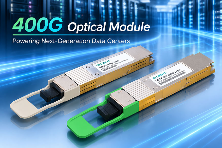
| 400G | QSFP-DD, OSFP, QSFP112 | Approximately 8–12 W for many conventional datacom variants | High-density switching and AI fabrics |
| 800G | QSFP-DD, OSFP | Approximately 13–18 W for many conventional datacom variants | AI training clusters and high-capacity data centers |
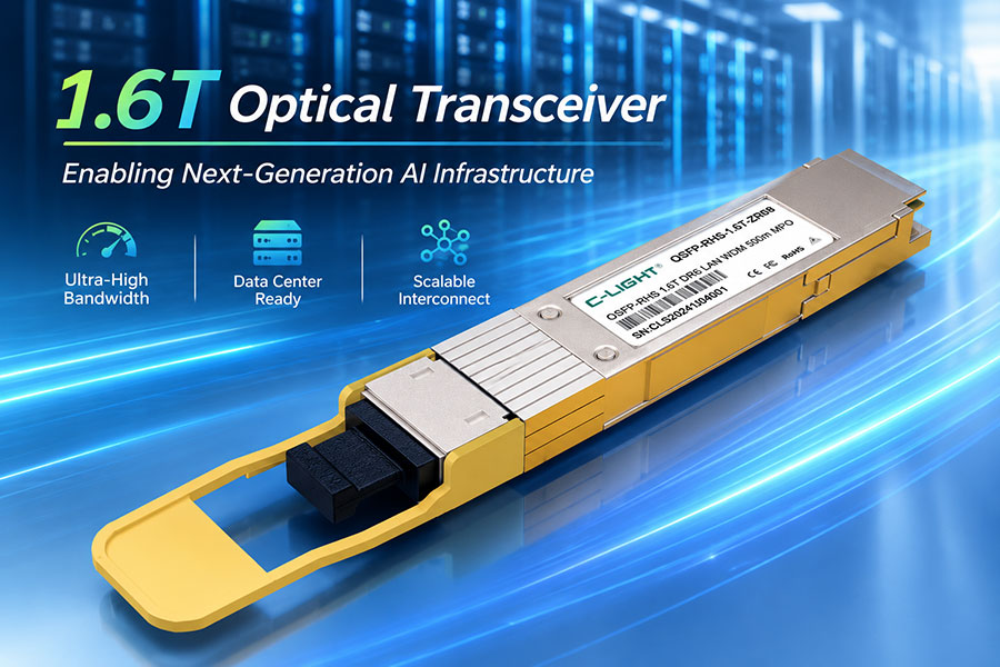
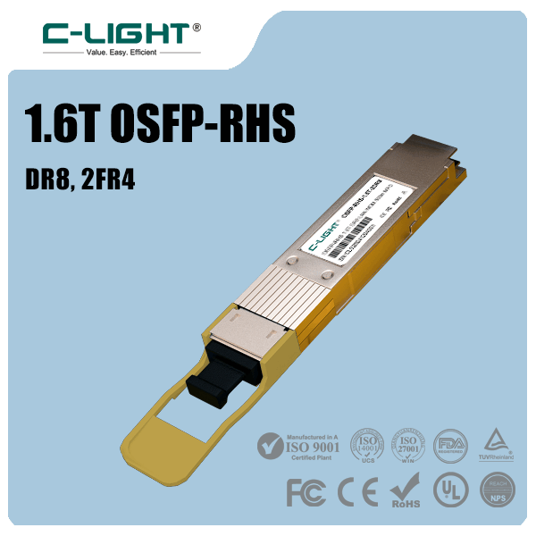
| 1.6T | OSFP and emerging high-speed form factors | Approximately 20–30 W for many retimed designs | Next-generation AI and cloud networking |
These ranges mainly represent common intensity-modulated direct-detection datacom modules. Long-reach coherent modules may consume substantially more power than short-reach DR or SR modules at the same aggregate data rate. Low-power LPO and LRO designs can also fall below conventional DSP-based module ranges.
3. What Determines Optical Module Power Consumption?
3.1 Digital Signal Processor
A DSP-based module may use digital equalization, signal recovery, retiming, lane mapping and other signal-processing functions to maintain link performance. At high baud rates, the DSP and associated high-speed circuitry can account for a substantial share of the module's total power.
DSP requirements vary by signaling rate, process technology, implementation and the amount of signal conditioning required. A module with a more advanced DSP may improve signal integrity, but its overall power must be evaluated alongside the optical engine and host interface.
3.2 Optical Transmitter and Receiver
The transmitter includes components such as lasers, modulators and driver circuits. The receiver commonly includes photodetectors and transimpedance amplifiers (TIAs). Their power depends on the optical architecture, required output power, receiver sensitivity, modulation format and target reach.
Short-reach VCSEL-based modules, single-mode silicon photonics designs and long-reach EML-based modules have different power profiles. Coherent modules add more complex optical and digital processing functions, so their power cannot be estimated reliably from data rate alone.
3.3 Retiming, Gearbox and Control Circuits
Retimers restore signal timing and amplitude, while gearboxes map data between different electrical and optical lane arrangements. Some products integrate these functions into the DSP; others use different implementations. Control interfaces, monitoring circuits and voltage regulation also contribute to total consumption.
3.4 Reach and Operating Conditions
Longer transmission distances may require higher optical output power, more sensitive receiver designs, optical amplification or more complex signal processing. Temperature can also affect laser behavior and circuit power. Some modules include thermal control functions that add to consumption under particular operating conditions.
4. Why Power Rises from 100G to 1.6T
Higher aggregate bandwidth requires faster electrical interfaces, more capable signal-processing circuits and optical components that support higher symbol rates or additional lanes. The module must preserve signal quality while operating within its specified electrical, optical and thermal limits.
| Generation | Common Architectural Trend | Power Design Challenge |
|---|---|---|
| 100G | Four 25G-class lanes in many QSFP28 implementations | Balancing lane performance, optical reach and compact packaging |
| 400G | Eight 50G-class lanes or four 100G-class optical lanes, depending on PMD | Managing DSP power and increased front-panel heat density |
| 800G | Eight 100G-class lanes or alternative supported lane mappings | Higher-speed signal conditioning and denser thermal loading |
| 1.6T | Eight 200G-class lanes in many emerging architectures | High-baud-rate signal integrity, DSP efficiency and advanced cooling |
Lane counts and signaling rates vary by PMD and host interface. For example, a 400G module using four 100G-class optical lanes does not have the same internal architecture as a design using eight 50G-class lanes. This distinction matters when estimating component power or comparing product efficiency.
5. DSP, LPO, LRO and CPO Power Differences
Optical architecture affects where signal processing takes place and how much power is consumed across the link. Conventional DSP-based pluggable modules prioritize signal conditioning and interoperability. LPO and LRO reduce some module-side processing, while CPO places optical engines close to the switch ASIC.
| Architecture | Power Characteristics | Key Engineering Consideration |
|---|---|---|
| DSP-based pluggable | Includes module-side DSP and associated circuitry | Strong signal conditioning and established serviceability; evaluate module power and heat. |
| LRO | Removes or reduces selected DSP functions; implementations may retain transmit-side retiming | Power savings depend on the precise retiming and receiver architecture. |
| LPO | Uses a more linear signal path to reduce module-side DSP power | Requires careful host signal integrity, channel design and interoperability validation. |
| CPO | Places optical engines near the switch ASIC to reduce electrical interconnect losses | System-level power, cooling, fiber management and serviceability must be considered. |
LPO does not automatically provide the best solution for every link. Its results depend on host SerDes performance, PCB channel loss, module implementation and operating conditions. CPO can improve link energy efficiency by reducing electrical path losses, but its advantages must be assessed at system level, including switch circuitry, optical engines, cooling and service requirements.
When comparing architectures, use consistent measurement boundaries. Comparing module-only watts with a system-level figure that includes host SerDes or cooling can produce misleading conclusions.
6. Power Consumption and Energy per Bit
Energy per bit relates module power to aggregate data rate. A useful first-order calculation is:
Energy per bit (pJ/bit) = Power (W) × 1,000 ÷ Data rate (Gb/s)
For example, an 800G module consuming 16 W has a module-level energy figure of approximately 20 pJ/bit when calculated using 800 Gb/s of nominal aggregate throughput.
A 1.6T module consuming 24 W yields approximately 15 pJ/bit using 1,600 Gb/s. In this example, the 1.6T module consumes more total power but uses less energy per nominal bit.
| Example Module | Assumed Power | Nominal Data Rate | Calculated Energy per Bit |
|---|---|---|---|
| 400G | 10 W | 400 Gb/s | 25 pJ/bit |
| 800G | 16 W | 800 Gb/s | 20 pJ/bit |
| 1.6T | 24 W | 1,600 Gb/s | 15 pJ/bit |
These are illustrative calculations, not measured performance claims for specific products. Actual energy efficiency depends on the defined throughput, coding overhead, traffic conditions and whether host SerDes or other system components are included.
7. Calculating Power at Switch and Data Center Scale
Individual modules may consume only several watts or a few tens of watts, but large port counts multiply the impact. Optical power can become a significant part of the switch's front-panel power and cooling budget.
Aggregate module power (W) = Number of installed modules × Power per module (W)
Consider a switch populated with 32 optical modules, each consuming 16 W:
Aggregate module power: 32 × 16 W = 512 W.
Continuous energy over 24 hours: 512 W × 24 h = 12.288 kWh.
Annual module energy at continuous full-load operation: approximately 4,485 kWh.
This calculation covers the optical modules only. It excludes the switch ASIC, fans, power-supply losses and other system components. Actual annual energy use will vary with module power, operating state and deployment utilization.
For facility planning, the IT equipment's electrical consumption and the additional energy needed by cooling and power infrastructure should be evaluated separately. A data center's Power Usage Effectiveness (PUE) can help estimate facility overhead, but it should not be treated as a fixed multiplier for every individual component without considering the site's operating conditions.
8. Thermal Management for High-Power Optical Modules
Nearly all electrical power consumed by an operating optical module ultimately becomes heat within the equipment and surrounding environment. Higher module power increases the thermal load near switch cages, where airflow and heatsink space may already be limited.
Key design considerations include:
Airflow direction and volume: Confirm that the switch platform supports the selected module's thermal requirements.
Module temperature limits: Check specified case-temperature and ambient operating ranges.
Port population: Validate thermal performance with the expected number and arrangement of active modules installed.
Heatsink and cage design: Ensure that mechanical fit and thermal contact meet the platform's requirements.
Liquid cooling: Evaluate system-level cooling options when rack and switch thermal density exceeds practical air-cooling limits.
Power headroom: Provision for maximum specified module power rather than relying solely on typical consumption.
A module's stated power does not guarantee that it will operate within temperature limits in every switch. Compatibility includes the host platform's airflow, module power class, firmware support and thermal design.
9. How to Reduce Optical Transceiver Power Consumption
9.1 Select the Appropriate Reach
Avoid specifying a long-reach or coherent module when a supported short-reach datacom optic meets the actual link budget. Match the optical interface to fiber type, distance, connector loss and required margin rather than choosing solely by data rate.
9.2 Evaluate Lower-Power Architectures
For suitable short-reach links, compare conventional DSP-based modules with LRO and LPO alternatives. Confirm host compatibility, reach, error performance and operating conditions before deployment.
9.3 Optimize Port and Link Design
Use the appropriate optical reach and lane configuration, consolidate unnecessary conversions where practical, and assess whether DAC, AOC or optical transceivers best fit each connection. Passive DACs consume no active power within the cable assembly itself, while active copper and AOC designs have their own power requirements and reach limits.
9.4 Validate Power at the System Level
Use datasheet maximum power for provisioning, then measure real module and system consumption under representative workloads. Include host SerDes, cooling and power-supply conversion losses when comparing complete architectures.
10. Power Monitoring and Troubleshooting
Digital Diagnostic Monitoring (DDM) and module management interfaces can provide useful telemetry, such as temperature, supply voltage, laser bias current and transmit or receive optical power, depending on the module and management implementation.
These readings can help identify abnormal operating conditions, but they do not necessarily report precise instantaneous module power. If power consumption is a concern, compare supported telemetry with the manufacturer's specification and, where appropriate, platform-level power measurements.
| Observed Condition | Possible Cause | Recommended Check |
|---|---|---|
| Module temperature is higher than expected | Restricted airflow, high ambient temperature or a heavily populated front panel | Review chassis airflow, module temperature limits and installed-module density. |
| Module power exceeds the expected budget | Different module variant, higher operating requirements or incorrect planning assumptions | Verify the part number and its typical and maximum power specifications. |
| Optical performance degrades as temperature rises | Thermal sensitivity, optical component behavior or host-platform limitations | Check temperature, optical power, error counters and the applicable module limits. |
| Switch rejects or disables a module | Unsupported power class, compatibility issue or platform policy | Check switch support, module qualification, firmware and platform power limits. |
11. Frequently Asked Questions
11.1 Do Higher-Speed Optical Transceivers Always Consume More Power?
Not necessarily in every comparison, but higher-speed modules often require more total power because of faster electrical signaling and more complex processing. Architecture, reach and implementation can significantly change the result.
11.2 Why Can Two 800G Optical Modules Have Different Power Ratings?
They may use different optical reaches, lane arrangements, DSP designs, modulators, laser technologies, form factors and thermal-management approaches. Coherent 800G modules generally have different power requirements from short-reach DR or SR datacom modules.
11.3 Is Lower Power Always Better?
Lower power is beneficial when the module still meets required reach, error performance, interoperability and environmental specifications. A low-power design that does not meet the link's requirements is not an effective replacement.
11.4 Does LPO Eliminate All Signal Processing?
No. LPO reduces or removes selected module-side DSP functions, but the host electrical interface and receiver still need to handle the signal correctly. The precise architecture varies by implementation.
11.5 How Much Power Should Be Reserved for a Module?
Use the maximum specified power and the host platform's module power-class requirements for provisioning. Typical consumption is useful for estimating operational energy, but it should not replace the maximum value in power and thermal design.
11.6 Does DDM Show the Exact Power Draw of an Optical Module?
Not necessarily. DDM commonly exposes temperature, voltage, bias current and optical measurements. Direct electrical power measurement or platform telemetry may be required to determine actual module consumption.
12. Conclusion
Optical transceiver power consumption is a system-design consideration that spans module selection, signal-processing architecture, link reach, port density and thermal management. As 400G, 800G and 1.6T interfaces become more common in AI and cloud networks, energy per bit is increasingly useful alongside absolute power.
Reliable planning starts with the exact product specification, a clear distinction between typical and maximum consumption, and a consistent measurement boundary. DSP-based optics, LPO, LRO and CPO offer different trade-offs in power, signal integrity, interoperability and serviceability. The best choice is the architecture that meets the network's performance requirements while remaining within the platform's electrical and thermal budgets.
Review module data rates, optical reach, compatibility and power requirements before finalizing the design.
Contact C-LIGHT >

 >
 >
 >
 >
 >
 >
 >