TEL:+86 132 6656 7067





An optical transceiver link budget determines whether enough optical power reaches the receiver after transmission through fiber, connectors, splices and other passive components. It is a fundamental design check for Ethernet, Fibre Channel, data center interconnect and telecom optical links. A valid budget helps engineers assess whether a link can meet its specified performance over the intended distance and under realistic operating conditions.
Nominal transmission distance alone does not establish link feasibility. Two links with the same length can have different losses because of fiber type, connector count, patch panels, splice quality and wavelength. The selected transceivers must provide sufficient optical power margin while also satisfying receiver overload limits and the applicable interface specification.
1. What Is an Optical Transceiver Link Budget?
An optical link budget compares the optical power available from the transmitter with the minimum power required by the receiver. The difference between transmit power and receiver sensitivity defines the nominal optical power budget when both specifications are expressed in compatible units.
Engineers then estimate the total loss of the optical path and compare it with the available budget. The remaining margin indicates how much additional loss the link can tolerate under the assumptions used in the calculation.
For example, if a transceiver specifies a minimum transmit power of -2 dBm and a receiver sensitivity of -10 dBm, the calculated budget is 8 dB. This does not mean the link can automatically support any distance corresponding to 8 dB of fiber loss: connector losses, splices, engineering margin and other applicable requirements must also be included.
2. Key Optical Link Budget Parameters
| Parameter | Definition | Role in the Calculation |
|---|---|---|
| Transmit power (Tx) | Optical power launched by the transmitter, specified in dBm | Defines the available launch power. Use the appropriate minimum or maximum value for the check being performed. |
| Receiver sensitivity | Minimum received optical power for the specified performance criterion | Defines the lower end of the receiver's operating range under stated test conditions. |
| Receiver overload | Maximum specified received optical power for compliant operation | Checks whether a short or low-loss link could deliver too much power. |
| Fiber attenuation | Optical power loss per unit distance, commonly expressed in dB/km | Estimates the loss accumulated over the fiber route. |
| Connector loss | Insertion loss at each mated connector pair or applicable connection point | Accounts for patch panels, equipment connections and intermediate interfaces. |
| Splice loss | Loss introduced by fusion or mechanical splices | Accounts for permanent joints in the optical path. |
| Engineering margin | Reserved allowance for uncertainty, aging, repairs or future degradation | Prevents the design from relying entirely on the nominal loss calculation. |
Use values specified for the exact transceiver variant and applicable optical interface. Minimum transmit power, receiver sensitivity and receiver overload are different limits, and confusing them can produce an unsafe or inaccurate design.
3. How to Calculate an Optical Link Budget
A practical link budget follows four steps: calculate the available optical budget, estimate the total path loss, subtract a suitable engineering margin, and check the received power against both receiver sensitivity and overload.
3.1 Calculate the Available Power Budget
Using minimum transmit power is a conservative approach for checking the receiver's low-power limit. For a standards-based link, use the transmit-power and receiver-sensitivity definitions specified for the relevant interface.
3.2 Calculate Total Optical Path Loss
Fiber loss is calculated from attenuation multiplied by route length. Connector and splice losses are added according to the actual optical path, including the number of mated pairs and joints. Include other components, such as passive splitters, filters or patching elements, where applicable.
3.3 Calculate the Remaining Margin
A positive remaining margin indicates that the calculated path fits within the chosen budget and reserve. A negative result means the design needs further investigation or a different combination of optics, fiber route or passive components.
3.4 Check Received Power
The estimated received power can be calculated as:
Check the result against receiver sensitivity and receiver overload. A link can have adequate power at the receiver's low end yet exceed the maximum permitted receive power when the path loss is very small. Minimum-loss and maximum-loss cases should both be considered where the applicable specification requires them.
4. Worked Example: A Single-Mode Fiber Link
Consider a hypothetical single-mode link with the following design assumptions. These values illustrate the calculation only and are not specifications for a particular transceiver.
| Input | Assumed Value |
|---|---|
| Minimum transmitter output power | -2 dBm |
| Receiver sensitivity | -10 dBm |
| Fiber length | 10 km |
| Assumed fiber attenuation | 0.35 dB/km |
| Connector loss allowance | 1.0 dB total |
| Splice loss allowance | 0.2 dB total |
| Reserved engineering margin | 2.0 dB |
Step 1: Available optical budget
-2 dBm − (-10 dBm) = 8 dB.
Step 2: Fiber loss
10 km × 0.35 dB/km = 3.5 dB.
Step 3: Total path loss
3.5 dB + 1.0 dB + 0.2 dB = 4.7 dB.
Step 4: Remaining margin after reserve
8 dB − 4.7 dB − 2 dB = 1.3 dB.
5. Fiber Attenuation and Transmission Distance
Fiber attenuation is wavelength- and fiber-dependent. Single-mode fiber is commonly used for longer distances, while multimode fiber is widely used for short-reach links inside data centers. The actual attenuation limit should be selected for the installed fiber and the operating wavelength.
| Fiber Type or Wavelength Region | Illustrative Attenuation Range | Design Consideration |
|---|---|---|
| Multimode fiber near 850 nm | Often around 2–3.5 dB/km, depending on fiber specification | Modal bandwidth and the specified SR interface can limit reach before attenuation alone becomes the deciding factor. |
| Single-mode fiber near 1310 nm | Often around 0.3–0.4 dB/km | Commonly used for many DR and LR datacom interfaces, subject to the specified PMD. |
| Single-mode fiber near 1550 nm | Often around 0.18–0.25 dB/km | Low attenuation supports longer links, but dispersion, optical amplification and interface limits may become important. |
These figures are general planning examples rather than universal cable limits. Installed fiber performance depends on cable specifications, wavelength, environmental conditions and measurement method.
Optical reach is not determined by attenuation alone. At high data rates, chromatic dispersion, modal bandwidth, receiver performance, reflections and signal-to-noise requirements may limit the distance even when the calculated optical power budget appears adequate.
6. Connector, Splice and Passive Component Losses
Every connection in the optical path can introduce insertion loss. A link with multiple patch panels or cross-connects may consume a significant portion of its available budget before fiber attenuation is considered.
Connector pairs: Count the actual mated interfaces along the route and use an appropriate insertion-loss allowance for each pair.
Splices: Include the number of splices and the expected loss per splice.
Patch panels: Account for all intermediate connections, not just the two equipment-side connectors.
Passive optical components: Add specified insertion loss for splitters, filters, multiplexers or other elements in the path.
Connector cleanliness: Inspect and clean connectors using appropriate procedures before mating them.
Do not double-count a connection if the chosen link-loss specification already includes it. The calculation should reflect the actual physical path and a clearly defined loss model.
7. Link Budget vs. Optical Power Budget
The terms “link budget” and “optical power budget” are often used interchangeably in transceiver selection, but their intended scope can differ.
| Term | Typical Meaning | Primary Use |
|---|---|---|
| Optical power budget | Difference between specified transmitter power and receiver sensitivity | Determines the nominal optical loss that can be tolerated under the defined specifications. |
| Link budget | System-level assessment of available power, path losses, margin and applicable performance constraints | Checks whether the planned optical link can operate within its requirements. |
| Engineering margin | Reserved allowance for uncertainty or degradation | Provides protection against a design that only works under ideal assumptions. |
For procurement and deployment, it is useful to calculate the nominal power budget first and then document all path-loss assumptions, margin requirements and other optical-performance constraints separately.
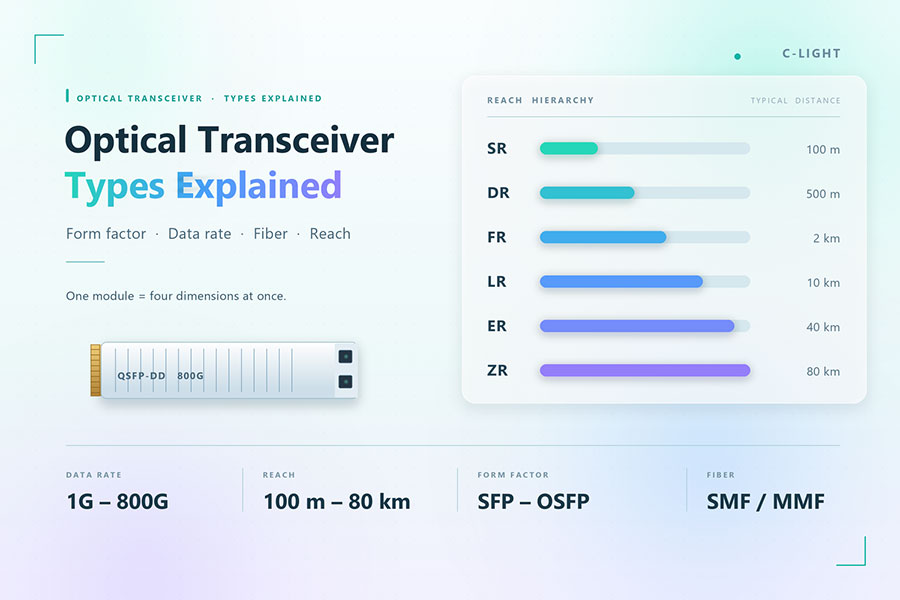
8. Link Budget Requirements for SR, DR, FR and LR Optics
Different optical interface families are designed for different media and distances. Their reach labels should not be treated as interchangeable specifications, even if their modules share the same form factor or aggregate data rate.
| Optical Interface Family | Typical Medium | Common Design Context | Important Checks |
|---|---|---|---|
| SR | Multimode fiber | Short-reach data center links | Fiber grade, wavelength, modal bandwidth, connector and specified reach. |
| DR | Single-mode fiber | Direct-detection links over specified data center distances | Fiber loss, connector loss, lane mapping and the relevant DR specification. |
| FR | Single-mode fiber | Intermediate-reach links using the specified optical interface | Wavelength arrangement, reach, power budget and receiver limits. |
| LR | Single-mode fiber | Longer-reach datacom links | Route loss, dispersion-related limits, connector count and optical margin. |
| ER / ZR and other extended-reach variants | Usually single-mode fiber | Longer-reach applications with interface-specific requirements | Check the exact standard or vendor specification, including power, dispersion and any amplification requirements. |
Exact distances and power limits depend on the specific standard and product variant. A nominal reach value should not replace a calculation based on the module's specified transmitter power, receiver sensitivity, overload limit and link requirements.
9. Receiver Sensitivity, Overload and Optical Margin
Receiver sensitivity is the minimum input power required to achieve the specified performance under defined test conditions. Receiver overload is the upper receive-power limit for compliant operation. Both are important when validating a link.
For a conservative low-power check, use minimum transmitter power and maximum expected path loss. For an overload check, use the highest applicable transmitter power and minimum expected path loss. Confirm that both cases fall within the receiver's specified operating range.
The receiver's sensitivity specification is associated with a defined bit error performance, test setup and interface. A sensitivity value should not be treated as a universal threshold independent of modulation format, FEC behavior or the applicable standard.
10. Common Optical Link Budget Mistakes
Using typical transmit power instead of the specified minimum: This can overestimate the available budget for a worst-case check.
Ignoring connector and patch-panel losses: The fiber length may be correct while the total path-loss estimate is incomplete.
Confusing dBm with dB: dBm represents an absolute power level; dB represents a relative difference or loss.
Ignoring receiver overload: Short links can have excessive receive power even when the power budget is sufficient.
Assuming attenuation defines reach: Dispersion and other interface limits may restrict transmission distance.
Using generic fiber-loss values without checking the cable specification: The correct assumptions depend on fiber type and wavelength.
Forgetting the engineering margin: A link with almost no reserve may be vulnerable to normal variations or future repairs.
Mixing incompatible specifications: Transmit power, sensitivity and reach values must refer to the same compatible interface and operating conditions.
11. Verifying a Link Budget in the Field
After installation, optical power measurements can be used to compare actual link behavior with the design calculation. The measurement point, test wavelength and instrument accuracy should be appropriate for the interface under test.
Verify the transceiver model, optical interface and specified operating wavelength.
Inspect and clean connectors before connecting test equipment or the installed fiber route.
Measure transmit and receive optical power where the device and test setup permit.
Compare measured receive power with the module's sensitivity and overload limits.
Review error counters and FEC statistics, where applicable, to assess transmission performance beyond raw optical power.
Recalculate the path loss if measurements differ materially from the expected values.
DDM/DOM telemetry can provide useful transmit power, receive power and temperature readings, depending on the transceiver and host platform. These readings support troubleshooting, but they may have measurement tolerances and do not replace calibrated optical test equipment where precision measurements are required.
12. Frequently Asked Questions
12.1 What Is the Formula for an Optical Transceiver Link Budget?
Available optical power budget equals transmitter output power minus receiver sensitivity, with both values expressed in dBm. The remaining margin is the available budget minus total path loss and the reserved engineering margin.
12.2 What Is the Difference Between dB and dBm?
dBm is an absolute optical power level referenced to 1 milliwatt. dB is a relative ratio used for gain, attenuation or differences between power levels. Link-budget calculations subtract dBm values to obtain a result in dB.
12.3 Does a Higher Optical Power Budget Always Mean Longer Reach?
No. A higher budget can allow more optical loss, but the specified reach may also be limited by dispersion, modal bandwidth, signal quality, receiver design and other requirements of the optical interface.
12.4 How Much Engineering Margin Should a Link Have?
The required margin depends on the network design, applicable standards, route uncertainty, expected aging and maintenance practices. Use the relevant system design rules and product specifications rather than applying one universal margin to every link.
12.5 Can a Link Exceed Receiver Overload Even if Its Power Budget Is Valid?
Yes. The available power budget primarily checks whether enough power reaches the receiver. A separate maximum-power check is needed to confirm that the receiver is not exposed to excessive input power.
12.6 Can DDM Readings Confirm the Entire Link Budget?
DDM can help validate operating optical power at supported measurement points, but it does not automatically account for every path component or all signal-quality limits. Combine telemetry with route-loss records, device specifications and appropriate optical measurements.
13. Conclusion
An optical transceiver link budget provides a quantitative way to evaluate whether a planned fiber connection has sufficient optical power and engineering margin. Reliable calculations require the correct transmitter and receiver specifications, realistic fiber attenuation, complete connector and splice losses, and checks against both receiver sensitivity and overload.
For 100G, 400G, 800G and other high-speed optical links, power-budget calculations should be combined with the relevant interface requirements for dispersion, signal quality and error performance. A documented link budget, followed by field verification, helps prevent avoidable link failures and supports dependable network operation.
Confirm the interface standard, transmission distance, fiber type, connector count and optical power specifications before deployment.
Contact C-LIGHT >

 >
 >
 >
 >
 >
 >
 >