TEL:+86 132 6656 7067





Optical link budget calculations determine whether a fiber connection can deliver sufficient optical power to the receiver while preserving the required operating margin. For 100G, 400G, 800G, and 1.6T networks, accurate planning must account for transmitter output, receiver sensitivity, fiber attenuation, connector losses, passive components, and transmission penalties.
1. What Is an Optical Link Budget?
An optical link budget is the balance between the optical power available from a transmitter and the losses and performance penalties encountered before the signal reaches the receiver. It helps engineers evaluate whether a proposed fiber route can operate within the limits of the selected transceivers and optical interface.
Every optical link has a finite power budget. The transmitter provides optical power, while the fiber, connectors, splices, patch panels, and passive components reduce the power reaching the receiver. The receiver must receive a suitable signal level to meet the specified performance requirements.
For a point-to-point optical link, the available optical power budget is typically calculated from the minimum specified transmit power and the receiver sensitivity. The resulting value indicates the maximum loss that can be tolerated under the applicable assumptions. The actual deployment must also account for optical path penalties and an appropriate engineering margin.
Optical link budget calculations are relevant to short-reach data center connections, campus networks, metro links, and longer-distance optical transport. However, the calculation method and additional performance requirements depend on the optical technology being deployed.
2. The Basic Optical Link Budget Formula
The first step is to determine the available power budget from the transmitter and receiver specifications.
For example, if a transceiver specifies a minimum transmit power of −3 dBm and a receiver sensitivity of −12 dBm, the available power budget is:
This means the link has a nominal 9 dB power budget under these stated assumptions. The number is illustrative; actual transmit power and receiver sensitivity must come from the specifications for the selected optical interface.
The next step is to calculate the total expected link loss and compare it with the available budget.
A practical power-margin calculation is:
If the remaining margin is positive, the link meets the selected budget calculation with the specified reserve included. If the result is negative, the proposed link does not meet the design target and must be reassessed.
3. Key Parameters Used in the Calculation
| Parameter | Unit | Role in Link Design |
|---|---|---|
| Minimum transmit optical power | dBm | Defines the low-end transmitter output used in a conservative power-budget calculation. |
| Receiver sensitivity | dBm | Defines the minimum received signal level at which the receiver meets the specified performance conditions. |
| Fiber attenuation | dB/km | Represents power loss per kilometer at the relevant wavelength and fiber conditions. |
| Fiber length | km | Determines the fiber attenuation component of the total link loss. |
| Connector loss | dB | Accounts for losses at mated optical connector interfaces along the link. |
| Splice loss | dB | Accounts for losses introduced by fiber splices. |
| Passive component loss | dB | Accounts for additional losses from patch panels, splitters, muxes, demuxes, and other components where applicable. |
| Optical path penalty | dB or specification-specific metric | Accounts for applicable transmission impairments not already included in the link budget model. |
| Engineering margin | dB | Provides reserve for uncertainty, aging, maintenance, and expected changes in operating conditions. |
Use consistent units throughout the calculation. Transmit power and receiver sensitivity are expressed in dBm, while losses and the power budget are expressed in dB. Because dBm is an absolute power level and dB is a ratio, the budget is calculated by subtracting the two dBm values.
4. Calculate Fiber Attenuation
Fiber attenuation is the power lost as an optical signal propagates through the fiber. The amount depends on fiber type, wavelength, cable quality, and installation conditions. For a basic calculation, fiber loss can be estimated from the attenuation coefficient and total fiber length.
For example, assume a 10 km single-mode fiber route has a planning attenuation value of 0.35 dB/km at the relevant wavelength:
The estimated fiber attenuation is 3.5 dB. This value is an illustrative planning assumption, not a universal specification. The actual attenuation should be based on the fiber cable specification, wavelength, measured link characteristics, and applicable interface requirements.
For short-reach links, connector and patching losses can represent a substantial portion of the total loss. For long fiber routes, attenuation becomes more significant, and the design may also need to consider dispersion and other transmission penalties.
5. Calculate Connector, Splice, and Passive Component Losses
Fiber links contain more than the fiber cable itself. Each optical connection or passive component may introduce additional insertion loss. These losses must be included in the design estimate instead of calculating the link from distance alone.
Connector loss
Connector loss depends on connector quality, alignment, end-face condition, cleanliness, and the characteristics of the mated pair. Estimate the loss using the applicable component specifications or measurements, and count each mated interface in the actual path.
Splice loss
Splices used to join fiber sections introduce additional attenuation. The total estimated splice loss is calculated by multiplying the number of splices by the expected loss per splice. The applicable allowance should reflect the installation method and measured or specified values.
Passive component loss
Optical links may include patch panels, wavelength-division multiplexing equipment, splitters, filters, or other passive components. Their insertion losses should be added according to the specific optical path.
For example, a DWDM link using multiplexers and demultiplexers may have substantially different loss characteristics from a direct fiber connection. Component specifications should be reviewed before the overall link budget is finalized.
6. Worked Example: A 10 km Single-Mode Fiber Link
Consider an illustrative 10 km optical link with the following assumed parameters. These values demonstrate the calculation method and are not specifications for a particular transceiver or Ethernet physical layer.
| Parameter | Assumed Value | Calculation |
|---|---|---|
| Minimum transmit power | −3 dBm | From the illustrative transmitter specification |
| Receiver sensitivity | −12 dBm | From the illustrative receiver specification |
| Available power budget | 9 dB | −3 − (−12) |
| Fiber length | 10 km | Specified route length |
| Fiber attenuation | 0.35 dB/km | 10 × 0.35 = 3.5 dB |
| Connector and patching loss | 1.0 dB | Illustrative allowance for the complete path |
| Splice loss | 0.2 dB | Illustrative allowance |
| Other passive component loss | 1.0 dB | Illustrative allowance for components in the path |
| Engineering reserve | 2.0 dB | Chosen reserve for this example |
First, calculate total physical link loss:
Next, subtract the physical link loss and engineering reserve from the available power budget:
The example leaves 1.3 dB beyond the assumed engineering reserve. Under this simplified model, the link passes the power-budget calculation. Actual approval still depends on the selected transceiver's complete specifications, applicable optical penalties, receiver input limits, and any other required interface conditions.
7. Power Budget vs. Maximum Optical Reach
The available power budget helps determine whether sufficient optical power can reach the receiver, but it does not independently establish the maximum transmission distance. Two interfaces with different receiver sensitivities or transmitter power ranges can have different budgets, even if their nominal reach ratings appear similar.
| Design Factor | What It Determines | Why It Matters |
|---|---|---|
| Optical power budget | Available power relative to the receiver sensitivity | Establishes the basic allowance for link attenuation under specified conditions |
| Maximum channel insertion loss | The permitted insertion loss of the optical channel under the applicable specification | May include detailed transmitter, receiver, and channel constraints not captured by a simple power budget |
| Maximum receiver input power | The upper acceptable optical input level | Prevents a design that has sufficient power but exceeds the receiver's allowed input range |
| Chromatic dispersion | Signal distortion accumulated over the fiber path | May limit reach even when receive power remains acceptable |
| Optical return loss and reflections | Reflected light and its effect on the link | Important for interfaces with applicable reflection or return-loss requirements |
| OSNR and nonlinear effects | Signal quality in amplified and coherent optical systems | May be decisive in DWDM systems where power levels alone do not establish reach |
| FEC and error performance | Ability to maintain the specified error rate | Confirms that the link meets the actual performance target rather than only a power threshold |
The maximum distance must be based on the specified optical interface and its supported operating conditions. Increasing transmitter power or adding amplification does not automatically extend reach if dispersion, OSNR, nonlinear effects, or receiver input limits become the controlling factor.
8. Optical Link Budget Considerations for 100G, 400G, 800G, and 1.6T
High-speed Ethernet interfaces use different optical architectures, and their link-budget requirements cannot be inferred from data rate alone. The applicable standard or product datasheet defines the transmitter and receiver parameters, channel loss constraints, and other optical performance requirements.
| Network Interface | Examples of Optical Architecture | Link-Budget Considerations |
|---|---|---|
| 100G | SR4, DR, LR, ER-family interfaces | Verify wavelength, fiber type, lane configuration, supported reach, and the exact power and channel-loss specifications. |
| 400G | SR8, DR4, FR4, LR4, ER4-family interfaces | Distinguish parallel optics from wavelength-multiplexed designs and check the corresponding connector and channel requirements. |
| 800G | SR8, DR8, 2×DR4, 2×FR4, coherent ZR-family designs, among others | Confirm the exact physical-layer interface, fiber configuration, module specifications, and whether optical line-system parameters apply. |
| 1.6T | Selected 200G-per-lane optical architectures | Verify the exact lane mapping, optical architecture, supported reach, connector configuration, and module-specific limits. |
For a short-reach parallel optical module, connector type, polarity, individual lane performance, and fiber continuity can be important. For a wavelength-multiplexed module, the wavelength plan and multiplexing component losses must also be evaluated. For coherent ZR and ZR+ links, optical signal-to-noise ratio, amplifier noise, dispersion tolerance, and supported transmission modes can be more important than a simple end-to-end power budget.
At higher speeds, verify the behavior of all optical lanes where applicable. A link can show sufficient aggregate receive power while one lane operates abnormally or error performance falls outside the intended limits.
9. Optical Link Budget for Coherent and DWDM Systems
Coherent optical systems are often used for extended-reach data center interconnects and metro or regional DWDM networks. These links may include optical amplifiers, wavelength multiplexers, demultiplexers, filters, and intermediate optical nodes.
In such designs, an end-to-end power calculation remains useful for evaluating attenuation and receiver input levels, but it is not a complete reach analysis.
Important additional parameters include:
Optical signal-to-noise ratio (OSNR): Check that the signal quality at the receiver meets the requirement for the selected modulation and FEC mode.
Amplifier gain and noise figure: Account for the signal gain and noise introduced by optical amplifiers across the transmission path.
Wavelength plan: Confirm that the transceiver's tuning range, channel spacing, and optical filters match the line system.
Dispersion tolerance: Verify the module's supported operating range for chromatic dispersion and other relevant impairments.
Nonlinear effects: Consider the optical power and fiber conditions under which nonlinear transmission impairments may become significant.
Receiver operating range: Confirm both the required minimum signal level and the maximum supported input level.
For amplified DWDM links, a design should be validated against the applicable optical system specification and the performance limits of the complete transmission path. A calculation based only on minimum transmitter power and receiver sensitivity may incorrectly predict that a route is suitable.
10. Common Optical Link Budget Errors
| Common Error | Why It Causes Problems | Recommended Practice |
|---|---|---|
| Using typical rather than guaranteed minimum transmit power | Overestimates the power available under worst-case operating conditions | Use the relevant minimum transmitter specification for the chosen calculation method. |
| Ignoring receiver overload limits | A receiver may be exposed to too much optical power even though the loss budget is positive | Verify both minimum sensitivity and maximum input specifications. |
| Calculating fiber loss without connector losses | Underestimates the loss of the installed transmission path | Include every connector pair, splice, patch panel, and passive component in the path. |
| Using an arbitrary attenuation coefficient | May misrepresent actual fiber loss at the operating wavelength | Use cable specifications and measurements appropriate to the fiber and wavelength. |
| Assuming reach from distance alone | Ignores the optical budget and non-power transmission limitations | Verify that the complete physical layer supports the planned route and system configuration. |
| Applying the same calculation to coherent and direct-detection links | Misses OSNR, dispersion, amplifier, and related constraints | Use the system design method defined for the specific optical architecture. |
| Leaving insufficient reserve | Small changes in loss or operating conditions can consume the remaining margin | Choose an engineering reserve appropriate to the deployment and its uncertainty. |
| Double-counting penalties or component losses | Produces a misleading assessment of the available margin | Document each allowance and confirm which effects are already included in the applicable specification. |
11. Practical Link Budget Verification Before Deployment
After completing the calculation, validate the result against the actual fiber installation and selected transceivers. A theoretical budget is a planning tool; the installed link still requires physical inspection and, where appropriate, measurements.
Confirm transceiver specifications: Record exact part numbers, optical interfaces, minimum transmit power, receiver sensitivity, maximum receiver input power, and required reach.
Document the fiber route: Record cable length, fiber type, connectors, patch panels, splices, and passive optical components.
Calculate the expected loss: Combine the relevant fiber and component losses without double counting.
Reserve sufficient margin: Account for applicable optical path penalties and an engineering reserve appropriate to the link.
Check the receiver input range: Confirm the expected optical power remains both high enough and low enough for the receiver specifications.
Measure the installed path: Use suitable optical power and loss testing equipment where required, and compare results with the expected values.
Validate live diagnostics: Review Tx/Rx power, lane readings where available, module temperature, interface errors, and FEC statistics as supported by the platform.
Test operational stability: Verify link status and sustained traffic performance under representative operating conditions.
When measurements disagree with the calculated budget, inspect the optical connectors, confirm the measurement reference and instrument accuracy, verify the actual route and passive components, and check the transceiver diagnostics at both endpoints. If the power budget appears adequate but the link still performs poorly, investigate other relevant physical-layer constraints.
12. Frequently Asked Questions
12.1 How is an optical link budget calculated?
Subtract the receiver sensitivity in dBm from the minimum transmitter power in dBm to calculate the nominal available power budget in dB. Calculate fiber and component losses, then account for applicable optical penalties and an engineering reserve to determine the remaining margin.
12.2 What is the difference between dBm and dB?
dBm expresses absolute optical power relative to one milliwatt, while dB expresses a ratio or difference, such as attenuation or power budget. Subtracting receiver sensitivity in dBm from transmit power in dBm produces a value in dB.
12.3 Does a positive remaining margin guarantee a working optical link?
No. A positive margin means the link passes the stated power-budget calculation, assuming its inputs and model are valid. The complete interface must also meet receiver input limits, optical penalties, dispersion requirements, OSNR requirements where applicable, FEC behavior, and other specified performance conditions.
12.4 How much engineering margin should be reserved?
There is no single reserve that suits every link. The appropriate margin depends on the interface specification, uncertainty in loss estimates, connector and maintenance conditions, expected changes over time, and deployment requirements. Use a documented design criterion rather than an arbitrary value.
12.5 Can optical link budget determine the exact maximum distance?
Not by itself. Fiber attenuation and component losses help determine whether sufficient optical power can reach the receiver, but maximum reach may also be constrained by dispersion, signal quality, modulation, FEC, and the specified physical layer. Use the applicable interface specification and product datasheet.
12.6 Is the link budget calculation different for 400G and 800G transceivers?
The basic power-budget arithmetic is similar, but the optical parameters and applicable constraints differ by interface type. A 400G or 800G module may use parallel optics, wavelength multiplexing, or coherent transmission, each requiring the appropriate optical and system-level checks.
13. Summary
Optical link budget calculations are a core part of planning reliable fiber connectivity. By combining transmitter power, receiver sensitivity, fiber attenuation, connector losses, splice losses, passive component losses, and engineering margin, network designers can evaluate whether a proposed optical path meets its basic power requirements.
For high-speed data center networks, the calculation must be matched to the exact physical-layer specification. 100G, 400G, 800G, and 1.6T modules can differ substantially in lane architecture, modulation, connector configuration, reach, and receiver characteristics. Coherent and DWDM systems also require additional analysis of OSNR, amplification, and transmission impairments.
A sound deployment process combines a documented calculation with fiber inspection, optical measurements, transceiver diagnostics, and end-to-end link testing. This approach helps identify insufficient margin, avoid incompatible optical designs, and improve network reliability before production deployment.
Planning a high-speed optical deployment?
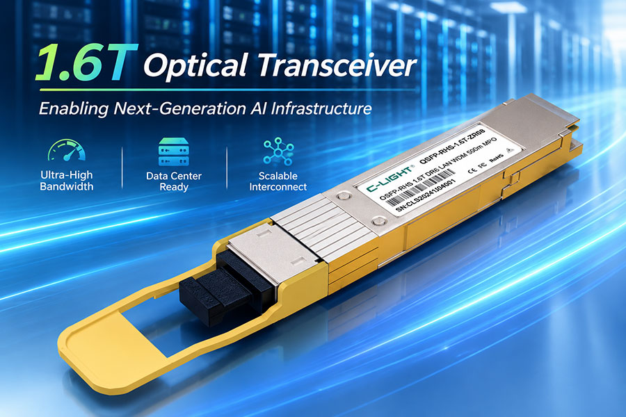
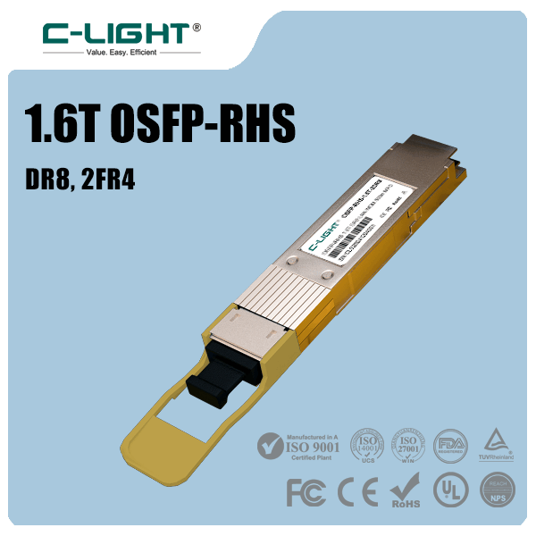
Review the 400G QSFP-DD, 800G OSFP, and 1.6T OSFP-RHS optical transceiver options, and confirm their link requirements against your fiber infrastructure.
Contact C-LIGHT >

 >
 >
 >
 >
 >
 >
 >