TEL:+86 132 6656 7067





In an AI training cluster, network bandwidth determines how efficiently accelerators exchange gradients, synchronize model parameters and distribute intermediate data. Adding GPUs increases computational capacity, but it also increases the volume of information that must move between them. When communication cannot keep pace with computation, accelerators may spend more time waiting for data, and additional hardware delivers less benefit than expected.
AI data center bandwidth planning therefore requires more than multiplying the number of servers by a network interface's nominal speed. The design must account for collective communication patterns, the ratio of endpoint bandwidth to switch capacity, oversubscription, congestion behavior, link utilization and the physical reach of each connection. Ethernet or InfiniBand fabrics, high-speed optical transceivers and the underlying fiber plant must be sized as one system.
1. Why AI Workloads Change Network Bandwidth Planning
Conventional enterprise applications often produce traffic that varies by user activity, request size and application behavior. Distributed AI training can generate more synchronized traffic patterns. Operations such as All-Reduce combine data across many accelerators, creating bursts of communication across a large portion of the cluster.
Bandwidth requirements also differ by workload. Training involves repeated synchronization and exchange of gradients or other distributed state. Inference may involve a mix of request traffic, retrieval operations and communication between model components. Large distributed inference systems can generate substantial inter-node traffic, but their requirements depend on model partitioning, batch size, sequence length and serving architecture.
| AI workload | Typical communication behavior | Bandwidth design priority |
|---|---|---|
| Distributed model training | Repeated synchronization and collective operations across many accelerators | High aggregate throughput, low congestion and predictable collective completion time |
| Tensor-parallel inference | Frequent exchanges between model partitions during inference | Low latency and high bandwidth between closely cooperating compute nodes |
| Pipeline-parallel workloads | Activations and intermediate results move between model stages | Capacity and latency aligned with stage placement and execution schedule |
| Data loading and checkpointing | Large transfers between compute nodes and storage systems | Aggregate throughput, burst handling and separation of storage and accelerator traffic where appropriate |
| Distributed inference serving | Request distribution, model sharding and inter-service communication | Traffic isolation, latency consistency and capacity under peak concurrency |
The same GPU count can therefore produce different network loads depending on the model and parallelization strategy. Bandwidth planning should begin with the communication graph and workload behavior, rather than assuming every accelerator generates the same sustained traffic at all times.
2. Scale-Up and Scale-Out Have Different Bandwidth Targets
AI systems commonly use multiple communication layers. Scale-up networking connects accelerators within a server or tightly integrated rack-level domain. Scale-out networking connects compute nodes across the broader cluster through switched fabrics. These layers serve different purposes and should not be sized using a single bandwidth assumption.
2.1 Scale-Up: Communication Among Closely Coupled Accelerators
Scale-up fabrics prioritize high bandwidth and low latency among accelerators that cooperate on the same model or computation. Depending on the platform, the interconnect may use proprietary accelerator links or other specialized high-speed interfaces. Their aggregate bandwidth figures may represent the sum of multiple links and directions, so they should not be compared directly with a single Ethernet port without aligning the measurement boundaries.
Scale-up capacity is often designed around a specific accelerator topology. The critical questions include how many peers each accelerator can reach, whether bandwidth is uniform between peers, and whether communication crosses a switch or multiple interconnect stages.
2.2 Scale-Out: Connecting Servers and Racks
Scale-out fabrics connect GPU servers through Ethernet or InfiniBand switches. This is where 400G and 800G optical connectivity is widely relevant, while 1.6T interfaces are emerging for next-generation high-density systems. Actual port speed depends on the network adapter, switch platform, optics and selected configuration.
Scale-out design must deliver enough aggregate capacity for communication between nodes while managing contention across shared uplinks. Even when each server has a high-speed network interface, the fabric can become oversubscribed if the uplink capacity is substantially lower than the sum of the endpoint rates.
3. Calculating Aggregate Network Bandwidth
A useful first step is to estimate the total line-rate capacity attached to the compute endpoints. If a cluster contains \(N\) nodes and each node has one network interface operating at \(R\) Gbit/s, the aggregate endpoint line rate is:
For example, a hypothetical cluster of 256 nodes, each with a 400 Gbit/s network interface, has an aggregate endpoint line rate of 102.4 Tbit/s. This is a planning baseline, not a guarantee that the fabric must carry 102.4 Tbit/s of simultaneous traffic in every scenario.
The required fabric capacity depends on the fraction of endpoint traffic that must cross the network at the same time, the traffic matrix, the topology and the acceptable oversubscription ratio. It also depends on whether traffic is local to a rack or crosses multiple network tiers.
3.1 Endpoint Rate Is Not Application Throughput
A 400 Gbit/s interface does not necessarily deliver 400 Gbit/s of application payload. Ethernet framing, packet size, protocol headers, congestion, transport behavior and workload characteristics affect usable throughput. Link rates also include the signaling capacity required by the physical and data-link layers.
For distributed training, average utilization alone may be misleading. A fabric with moderate average traffic can still experience short, synchronized bursts that create queue buildup and extend collective-operation completion time. Capacity models should therefore consider both average throughput and peak traffic patterns.
3.2 Oversubscription and Bisection Bandwidth
Oversubscription describes the relationship between the total bandwidth offered by a set of endpoints and the uplink bandwidth available to carry their traffic toward the rest of the fabric. A 2:1 ratio means the offered endpoint capacity is twice the relevant uplink capacity. Whether that ratio is acceptable depends on the traffic pattern and workload objectives.
Bisection bandwidth describes the capacity available when a network is divided into two halves and traffic must cross between them. It is useful for understanding large-scale communication, but a single bisection figure does not capture every path, hotspot or congestion condition in a real topology.
| Planning metric | What it indicates | What it cannot establish alone |
|---|---|---|
| Aggregate endpoint line rate | Total nominal network-interface capacity across nodes | Actual simultaneous traffic or application throughput |
| Oversubscription ratio | Relationship between endpoint capacity and shared uplinks | Whether a particular workload will experience congestion |
| Bisection bandwidth | Capacity available across a network partition | All path-specific bottlenecks and traffic hotspots |
| Measured utilization | Observed traffic relative to available link capacity | Whether short bursts or collective operations are being delayed |
4. How 400G, 800G and 1.6T Fit into AI Networks
Higher-speed ports increase the amount of traffic a physical interface can carry and can improve bandwidth density in the switch. The practical benefit depends on the full platform: switch radix, ASIC capacity, host interface speed, electrical signaling, optical module availability and the network's target topology.
| Port generation | Nominal aggregate rate | Typical planning role | Important design consideration |
|---|---|---|---|
| 400G | 400 Gbit/s | Established high-speed data center and AI cluster connectivity | Port count, link reach, existing switch support and upgrade cost |
| 800G | 800 Gbit/s | High-bandwidth AI fabrics and hyperscale networking | Host and switch support, optical power, thermal budget and lane architecture |
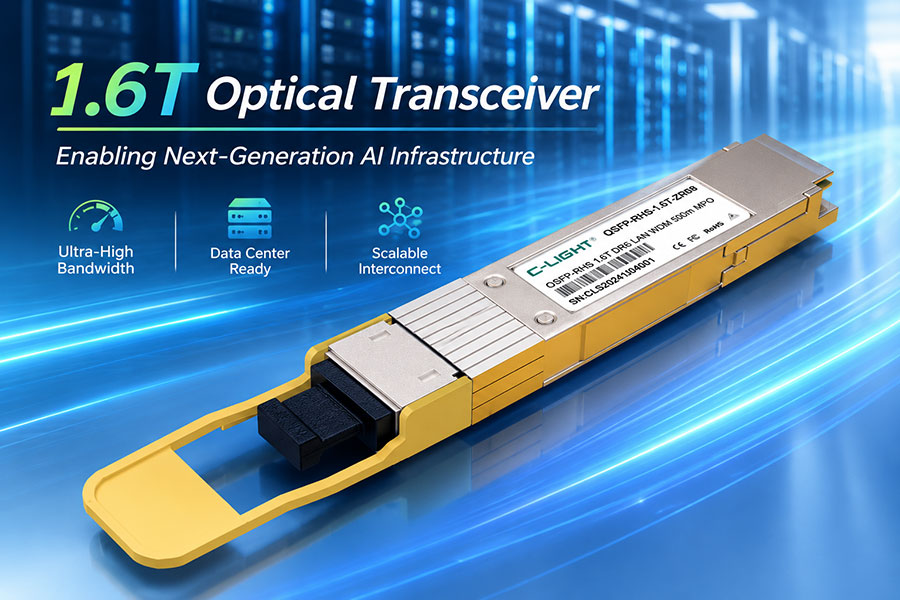
| 1.6T | 1.6 Tbit/s | Emerging next-generation platforms seeking greater bandwidth density | 200G-per-lane technology, signal integrity, thermal design and ecosystem maturity |
Moving from 400G to 800G doubles the nominal capacity of a port; moving from 800G to 1.6T doubles it again. This does not mean that application performance automatically doubles. If the workload is limited by compute, storage, software scheduling, congestion or a slower endpoint, increasing optical link speed alone may produce limited gains.
Higher port rates can also reduce the number of physical connections needed for a target aggregate capacity, depending on the switch design and topology. However, they introduce new requirements for electrical and optical lane speeds, power delivery, thermal management and qualification. The migration decision should balance capacity needs against platform readiness and total cost.
5. Optical Transceivers and the Physical Network Layer
Optical transceivers convert electrical signals from network equipment into optical signals for transmission over fiber and convert received optical signals back into electrical form. Their role becomes increasingly important as link rates and the distance between network devices exceed the practical reach of direct electrical connections.
The appropriate module depends on data rate, transmission distance, fiber type, connector arrangement and host compatibility. A bandwidth target alone is not enough to select the transceiver.
| Interconnect option | Typical application | Key trade-off |
|---|---|---|
| DAC | Short connections within racks or between nearby equipment | Low-cost passive or active copper connectivity, limited by reach and electrical characteristics |
| AEC | Short-reach connections where active electrical signal conditioning is useful | Can extend practical copper reach, with additional power and compatibility requirements |
| AOC | Short-to-moderate reach optical cabling with integrated optical ends | Factory-terminated assembly simplifies cabling but has fixed endpoint optics |
| Pluggable optical transceivers | Switch-to-switch, rack-to-rack and other optical network links | Flexible fiber infrastructure and reach options, with module power and compatibility considerations |
For optical links, transmission reach and fiber selection must match the intended application. Multimode fiber may suit some short-reach designs, while single-mode fiber supports a broad range of reaches and optical architectures. Connector type, fiber polarity, lane mapping and supported link configurations also need to align at both ends.
At 800G and 1.6T, the physical layer becomes more demanding. Electrical interfaces must preserve signal integrity at higher lane rates, while optical modules must meet their power, thermal and link-performance requirements. Compatibility must be verified across the transceiver, switch, firmware and relevant Ethernet or InfiniBand configuration.
6. Ethernet, RoCEv2 and InfiniBand Bandwidth Considerations
Ethernet and InfiniBand are both used in high-performance AI networking, but their deployment characteristics and operational models differ. Neither protocol eliminates the need for adequate physical capacity or a well-designed topology.
6.1 Ethernet with RoCEv2
RoCEv2 carries RDMA traffic over IP and Ethernet. It can support high-throughput, low-latency communication, but performance depends on end-to-end configuration, congestion management, traffic engineering and adapter capabilities. Loss management and congestion-control behavior require careful design, especially when synchronized collective traffic creates bursts.
6.2 InfiniBand
InfiniBand is widely used in high-performance computing and AI systems that require tightly integrated low-latency communication. Its fabric architecture, management and congestion behavior differ from Ethernet deployments. Bandwidth planning still needs to account for switch capacity, topology, link rates and the communication pattern of the accelerator workload.
Choosing between the two should reflect the required performance, software ecosystem, operational expertise, interoperability and cost. A nominal 800G link in one fabric is not automatically equivalent in end-to-end behavior to an 800G link in another fabric, because protocol overhead, congestion and topology affect the usable result.
7. Network Topology Determines How Much Bandwidth Is Usable
Leaf-spine designs are common in scale-out networks because they provide structured paths between endpoint racks and can be expanded by adding switches. The actual capacity available to a workload depends on the number of uplinks, the distribution of paths, routing behavior and whether the fabric is designed to be non-blocking for the target traffic pattern.
For AI clusters, topology should be evaluated against the communication graph of the workload. A design that performs well for uniform all-to-all traffic may behave differently when most traffic is concentrated among a subset of nodes or when many flows converge on the same destination.
Switch radix: determines how many high-speed ports are available for endpoint connections and fabric uplinks.
Path diversity: affects how traffic can be distributed across multiple links and switches.
Oversubscription: influences the capacity available during simultaneous inter-rack transfers.
Congestion control: helps manage traffic bursts and prevent persistent bottlenecks.
Failure behavior: link or switch failures can reduce available bandwidth and change traffic paths.
Designers should also account for operational headroom. A fabric sized only for its expected average traffic may struggle during synchronized training phases, recovery after failures or simultaneous checkpoint and storage operations.
8. Measuring Whether the Network Meets AI Bandwidth Requirements
Nominal link speed is a starting point. Validation should establish whether the complete fabric can deliver the throughput, latency consistency and communication performance required by the target workload.
| Measurement | Purpose | Interpretation |
|---|---|---|
| Per-link throughput | Measures data carried by individual links | Helps locate links approaching capacity limits |
| End-to-end throughput | Measures usable data rate between endpoints | Includes effects from protocol behavior, topology and congestion |
| Latency and tail latency | Measures communication delay and variability | Elevated or inconsistent latency can delay synchronization and collective completion |
| Packet loss and retransmissions | Identifies delivery problems and recovery overhead | May indicate congestion, physical-layer issues or configuration problems |
| Collective-operation time | Measures completion time for distributed communication primitives | Connects fabric behavior to actual training or inference performance |
| GPU utilization and stall indicators | Shows whether accelerators are waiting on data or other resources | Network symptoms should be correlated with compute, storage and software telemetry |
Testing should include representative message sizes, concurrency levels and communication patterns. A simple throughput test between two endpoints cannot establish the performance of a large multi-rack fabric under synchronized collective traffic. Conversely, low GPU utilization alone does not prove a network bottleneck; compute scheduling, data loading, memory pressure and software behavior can produce similar symptoms.
9. Planning Bandwidth for Future AI Cluster Expansion
AI network capacity is best planned as a staged expansion rather than a single port-speed decision. The initial deployment must meet current workload requirements, while the design should leave a practical path for increasing accelerator count and link capacity without replacing every component at once.
Define workload requirements: document accelerator count, parallelization strategy, communication patterns, expected utilization and acceptable job-completion time.
Model endpoint and fabric capacity: calculate aggregate line rate, uplink capacity, oversubscription and expected cross-rack traffic.
Choose link rates and media: align DAC, AEC, AOC or optical transceivers with distance, port density, power budget and platform support.
Validate the complete path: test adapters, switches, cables, optics and software using representative traffic patterns.
Plan for failure and growth: preserve capacity headroom for maintenance, failed links, new nodes and future bandwidth upgrades.
Track cost per useful throughput: consider transceivers, switches, power, cooling, cabling and the performance delivered to the workload.
The most useful long-term metric is not simply bandwidth per port. It is the amount of useful, predictable application throughput the network delivers within its cost, power and reliability constraints. A higher-speed optical interface is valuable when the surrounding architecture can use that capacity.
10. Conclusion
AI data center network bandwidth requirements are shaped by accelerator count, model-parallelism strategy, communication patterns, fabric topology and the capacity of each network layer. Scale-up and scale-out serve different roles, while oversubscription and congestion determine how much endpoint bandwidth remains available during coordinated workloads.
400G remains relevant to established high-speed deployments, 800G supports higher-capacity AI fabrics, and 1.6T is emerging as platforms adopt faster lane rates and greater bandwidth density. Selecting the right solution requires more than choosing the highest port speed: optical reach, media type, switch compatibility, thermal limits and end-to-end workload performance must all align.
11. Frequently Asked Questions
11.1 How much bandwidth does an AI data center need?
There is no universal figure. Requirements depend on the number of accelerators, the network rate per node, the model's communication pattern, topology and acceptable congestion. Aggregate endpoint line rate provides a useful starting point, but fabric capacity must be sized around expected traffic and performance targets.
11.2 Why is east-west traffic important in AI clusters?
East-west traffic carries data between servers and accelerators inside the data center. Distributed training and model-parallel inference can require frequent exchanges across many nodes, making inter-server bandwidth and congestion control central to workload performance.
11.3 Does an 800G network provide twice the application performance of a 400G network?
Not necessarily. An 800G port doubles nominal link capacity, but application performance also depends on endpoint capability, topology, congestion, protocol overhead, compute behavior and workload parallelism.
11.4 When should an AI network move from 800G to 1.6T?
The transition becomes relevant when 800G port density or aggregate fabric capacity no longer meets the target workload, and the switch, adapter, optical and thermal ecosystem supports 1.6T. A measured capacity shortfall and a platform-level cost assessment are stronger reasons than port speed alone.
11.5 Are optical transceivers required for every AI network connection?
No. DACs and AECs can serve suitable short electrical connections, while AOCs and pluggable optical transceivers provide optical connectivity for appropriate distances and deployment needs. The choice depends on reach, bandwidth, power, cabling density and equipment compatibility.
Building or expanding a high-bandwidth AI network?
Match optical transceiver speed, reach, fiber type and host compatibility to your switch architecture and deployment requirements.
Contact C-LIGHT >

 >
 >
 >
 >
 >
 >
 >